Inside INOPIA

Why INOPIA 

Water shortage can be defined as the condition, limited in space and time, characterized by insufficient availability of water resource with respect to the demand connected to it. According to the definition of Paulo and Pereira (2006) and Pereira et al (2019): “Water shortage is also a man-induced but temporary water imbalance including groundwater and surface water over-exploitation […]”. This concept is therefore applicable to water systems, which are set of infrastructures that capture and possibly store the water of one or more resources (surface and underground) and distribute it to different types of users (drinking water, irrigation, industrial, etc.). The shortage condition becomes particularly serious when dry situations occur for more or less prolonged periods of time. It is therefore evident that the identification of early-warning indicators of shortage conditions, meaning the inability of a system to meet the water needs of the connected users, must necessarily consider both the variability of meteorological forcing (including the medium-long term climatic trends) and the specific infrastructural and management characteristics of each system. The water supply systems can be extremely diversified both in terms of final user (systems for drinking water, irrigation, industrial or multiple purposes) and in terms of resource used (natural and artificial reservoirs, surface waters, aquifers alluvial, springs and treatment plants). INOPIA therefore wants to be a flexible generic decision support tool based on the calculation of the monthly mass balance (water volumes) of a multi-resource and multi-user water system consisting of water resources, water users, connections and management nodes elements. Considering time series of precipitation, available discharge observations, the needs of each macro users, the characteristics of the surface and underground reservoirs and the system management methods and level of interconnection, the tool estimates the water balance identifying the risk of deficit on each user/resource or on the entire system. The analysis of the historical relationship between the precipitation regime, resources availability and reconstructed deficits allows calibration of early-warning decision support of possible water crises as well as combined management, infrastructure and climatic scenarios.

Resources & Users Elements 

Inflows 

What is being represented 

The INFLOW element represents the discharge from a watershed that drains all the streams and rainfall to a common outlet such as the inflow of a reservoir or a river discharge at a given section.

The INFLOW element will supply time series of monthly mean discharge (m ³/s) to the WSS (water supply system).

INFLOWs can be connected to USER, RESERVOIR and MANAGEMENT elements.

Built-in model 

INFLOW element has a built-in model in INOPIA, called SPI-Q, reproducing monthly mean discharge based on precipitation anomalies. Such built-in model is a generic parsimonious rainfall-discharge model based on multi-regression on Standard Precipitation Index (SPI) (Romano et al. 2017; Romano et al. 2018), considering a hypotesis of stazionarity in the relation between precipitation anomalies at different time scale and the watershed hydrological response for a given month of the year.

When adding an INFLOW element to the WSS, the user is invited to indicate firstly a precipitation file, with one or more monthly cumulated precipitation time series (mm), and secondly a discharge file with observed discharge.

Single precipitation time serie may have missing values, but at least one value is needed for each month of the simulation timeline.

Differently, observed discharge can have missing values, but should have at least a known value for each month of the year. The quality of the resulting model (on estimated discharge) will highly depend on the depth of the observed discharge time serie. Depending on the case study, 20 to 30 years of observations may be necessary to obtain a fair calibration.

For each single precipitation time serie, INOPIA will estimate associated SPIs at different time scale (1,3 and 6 month) tipical of fast (e.g. surface runoff), medium (e.g. soil moisture) and slow (e.g. infiltration) hydrological processes at the watershed scale.

For each month of the year, a multi-linear regression is calibrated between the observed discharge and the mean SPIs values (among the station available in the precipitation file) of each scale:

\(Q(m_i )=a_0 (m)+a_{SPI1} (m) \cdot SPI1(m_i )+a_{SPI3} (m) \cdot SPI3(m_i )+a_{SPI6} (m) \cdot SPI6(m_i )\)

where \(Q(m_i)\) is the discharge for the month m, year i

\(SPI1(m_i )\), \(SPI3(m_i )\) and \(SPI6(m_i )\) are the Standard Precipitation Index (SPI) for the month m, year i based on the cumulative precipitation at 1, 3 and 6 months.

\(a_{SPI1} (m)\), \(a_{SPI3} (m)\) , \(a_{SPI6} (m)\) e \(a_0 (m)\) are the coefficients obtained from the multi-regression on SPI1, SPI3, SPI6 for the month m.

As a results, the INFLOW element will supply to the WSS continous monthly discharge on the precipitation timeline availability (e.g. having precipitation available for 1950-2020, supplying observed discharge for 1990-2015 will result in simulated discharge over 1950-2020).

The calibrated SPI-Q will thus be available for stochastic, scenarios and forecast simulation.

Input template 

When adding a new INFLOW element, the user will be asked to supply a precipitation file (with one station time series) and a discharge file (with on time serie of discharge)

The template input files for precipitation is available at the following link. The template input files for INFLOW discharge is available at the following link.

Optional input 

The discharge file can contain an optional sheet called ‘External’, with the results of an external modelling (as an alternative to the built-in model results). The template input files for INFLOW discharge with optional sheet is available at the following link.

If such optional sheet is present in the discharge file, the user will be asked to choose between built-in model and external model when running hindcast simulation.

Tip & tricks : ‘External’ sheet can be used to run the hindcast with the observed discharge over a period without missing data

Springs 

What is being represented 

As rainfall infiltration recharges the aquifer, pressure is placed on the water already present. This pressure moves water within the aquifer, and this water flows out naturally to the surface at places called SPRING. The SPRING element represents a surface natural discharge from an aquifer.

The SPRING element will supply time series of monthly mean discharge (m ³/s) to the WSS.

SPRINGs can be connected to USER, RESERVOIR and MANAGEMENT nodes.

Built-in model 

SPRING element has a built-in model in INOPIA, reproducing monthly mean discharge based on precipitation anomalies. Such built-in model is a generic parsimonious rainfall-infiltration-discharge model based on simple regression on Standard Precipitation Index (SPI) (Romano et al. 2017; Romano et al. 2018), considering a hypotesis of stazionarity in the relation between precipitation anomalies at different time scale and the aquifer hydrological response for a given month of the year.

When adding a SPRING element to the WSS, the user is invited to indicate firstly a precipitation file, with one or more monthly cumulated precipitation time series (mm), and secondly a discharge file with observed discharge.

Single precipitation time serie may have missing values, but at least one value is needed for each month of the simulation timeline.

Differently, observed discharge can have missing values, but should have at least a known value for each month of the year. The quality of the resulting model (on estimated discharge) will highly depend on the depth of the observed discharge time serie. Depending on the case study, 15 to 20 years of observations may be necessary to obtain a fair calibration.

For each single precipitation time serie, INOPIA will estimate associated SPIs at different time scale (from 1 to 24 month) also allowing infiltration delay through a monthly lag (from 0 to 6 month).

For each month of the year, a linear regression is calibrated between the observed discharge and the mean SPIs values (among the station available in the precipitation file) of each scale and lag:

\(Q(m_i )=a_0 (m)+a_{SPIX_\tau} (m) \cdot SPIX(m_i,\tau)\)

where \(Q(m_i)\) is the discharge for the month m, year i

\(SPIX(m_i,\tau)\) is the Standard Precipitation Index (SPI) for the month m, year i based on the cumulative precipitation at X months with \(\tau\) delay. The \(SPIX(m_i,\tau)\) is automatically selected by INOPIA as the scale and delay given the best results in term of Pearson correlation with the spring discharge.

\(a_{SPIX_\tau} (m)\) e \(a_0 (m)\) are the coefficients obtained from the regression.

As a result, the SPRING element will supply to the WSS continuous monthly discharge on the precipitation timeline availability (e.g. having precipitation available for 1950-2020, supplying observed discharge for 1990-2015 will result in simulated discharge over 1950-2020).

The calibrated built-in model will thus be available for stochastic, scenarios and forecast simulation.

Input template 

When adding a new SPRING element, the user will be asked to supply a precipitation file (with one station time series) and a spring discharge file (with on time serie of discharge)

The template input files for precipitation is available at the following link. The template input file for SPRING is available at the following link.

Optional input 

The spring discharge file can contain an optional sheet called ‘External’, with the results of an external modelling (as an alternative to the built-in model results). The template input files for SPRING discharge with optional sheet is available at the following link.

If such optional sheet is present in the discharge file, the user will be asked to choose between built-in model and external model when running hindcast simulation.

Tip & tricks : ‘External’ sheet can be used to run the hindcast with the observed discharge over a period without missing data

Wells 

What is being represented 

The WELL element simulates the behaviour of a wells-field pumping from a groundwater body in terms of the monthly maximum pumping rate that can be extracted from the groundwater body.

Built-in model 

The WELL element is not based on a built-in model that simulates the physical behavior of an aquifer. Consequently, no inter-annual variability nor internal mass balance is currently implemented in INOPIA WELL element. This is both a limitation and an advantage. A limitation because cumulated over-exploitation of a groundwater body is not explicitely monitored by INOPIA. An advantage because the WELL element does not need complex (and uncertain) parametrization of soil and groundwater hydrology which would limit its use and no a priori decision is made on the criteria to be considered for maximum pumping rate estimation (e.g. ecosystem services support, technological and infrastructure limits, concessions limits, sea water intrusion for coastal aquifer, ect …)

For the WELL element, a deficit condition arises when the sum of the water demands addressed to the resource for a given month is greater than the maximum exploitable volume.

To support the user in monitoring possible long-term overexploitation of a groundwater body exploited by a WELL element, its associated time serie plot proposes a 12 month moving average considering the sum of un-exploited resource and deficit (i.e. maximum pumping rate - demands).

Such time window (12 month) has been selected as the minimum covering the whole seasonality and may be under or over estimated depending on the actual groundwater body dynamic. Morevoer, if more wells-field are pumping in the same groundwater body, they may be aggregated in a single WELL element to keep such consideration meaningfull.

Input template 

When adding a new WELL element, the user will be asked to supply WELL monthly maximum pumping rate file

The template input file for WELL is available at the following link.

Reservoirs 

What is being represented 

The RESERVOIR element simulates a surface accumulation capacity, memorizing the evolution over time of the volumes stored in a reservoir, natural or artificial, on a monthly scale. It is based on the mass balance (volumes) calculated by considering as input data the inflow defined by one or more INFLOW or SPRING connected elements, the storage capacity, defined by a maximum and a dead volume, and the overall demand addressed to the element, relative to the current month.

Built-in model 

RESERVOIR element calculates the mass balance for the month t in the RESERVOIR according to the following input data: the volume stored at the end of the previous month \(V(t -1)\); the total inflow to the reservoir relative to the current month \(Q_{IN}(t)\); the volumes actually distributed by the RESERVOIR to all the USER connected \(SUP(t)\);

The mass balance of the reservoir is calculated as follows:

\(V(t,)= V(t -1) + \Sigma_j Q_{IN}(t,j)- \Sigma_u SUP(t,u)\)

where the sum on u is extended to all the USER elements (including ecological flow) connected with the RESERVOIR element and the sum on j to all the INFLOW or SPRING elements connected with the RESERVOIR element

:math:`V(t -1)` of the first month of simulation is taken from initial volume supplied in the RESERVOIR input file.

Input template 

When adding a new RESERVOIR element, the user will be asked to supply maximum, death and initial volume

The template input file for RESERVOIR is available at the following link.

Optional input 

The RESERVOIR input file can contain two optional sheet called Level and hypsographic.

The template input files for RESERVOIR with optional sheet is available at the following link

Level contains time serie of observed reservoir volume and will be used (if available) during time series plotting, providing an independent validation data for the hindcast simulation. hypsographic contains the hypsographic curve data (elevation above sea level (m (s.l.m.)) and corresponding volume (Mm ³)), allowing the definition of Alarm level for the early warning tool applied to the reservoir.

Alternative Water Sources (AWS)

What is being represented 

The Alternative Water Sources (AWS) element allows to implement non conventional resources characterized by a maximum exploitation rate that can be supplied for a given month. Some examples (not limited to) of alternative resources are desanalisation plant, treatment plant, rainfall harvesting or undersea fresh water captation.

Built-in model 

The AWS element considers monthly maximum exploitation rate and no inter-annual variability is currently implemented in INOPIA AWS element.

For the AWS element, a deficit condition arises when the sum of the water demands addressed to the resource for a given month is greater than the maximum exploitable volume.

Input template 

When adding a new AWS element, the user will be asked to supply AWS monthly maximum exploitation rate

The template input file for Alternative Water Sources (AWS) is available at the following link.

USER 

What is being represented 

The USER element represents a monthly water demand, as drinking water demand, irrigation or industrial needs.

Built-in model 

The USER element is currently not based on a built-in model that considers inter-annual variability in the monthly demands (e.g. irrigation demand based on soil moisture or drinking water demand based on population).

Each USER node is characterized by the following:

1.The monthly water demand
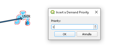
2.The priority level assigned by the user during the creation

The assigned priority (an integer between 1 and 10) is considered relatively to other USER elements priority possibly connected to one or more shared resource(s). For example, if two USERs with priority 1 and 2 respectively are connected to the same resource, the USER with priority 1 will be supplied in priority.

More about the connection rules can be found in Topology & connections rules

For the USER element, a deficit condition arises when the water demands for a given month is greater than available water in the connected resource(s), considering both priority and management rules (cf Management node)

Input template 

The template input file for USER is available at the following link.

Ecological flow 

What is being represented 

Ecological flow is considered within the context of the Water Framework Directive (WFD) as “an hydrological regime consistent with the achievement of the environmental objectives of the WFD in natural surface water bodies[…].”

In INOPIA, the Ecological flow element is considered as a USER element with the highest priority.

Built-in model 

The Ecological flow considers the monthly discharge supplied as input and will access connected resource(s) with first priority.

Input template 

The template input file for Ecological flow is available at the following link.

Topology & connections rules 

The design of a WSS can be a complex task depending on the number of the items and connections to be considered.

INOPIA intention is to simplify this task, using the collection of provided elements, adapting to every specific WSS.

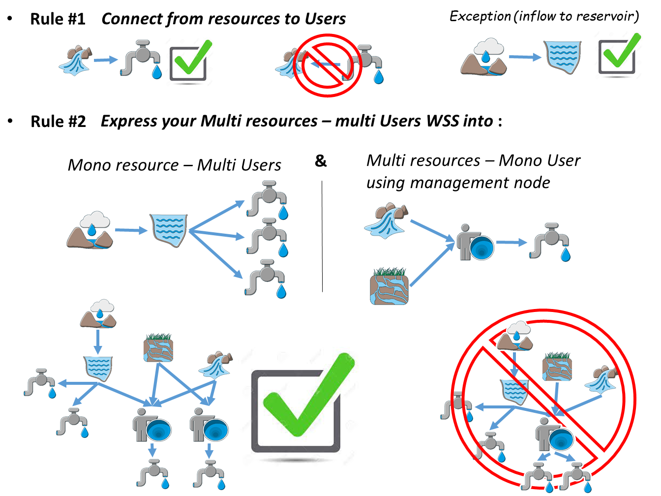
In order to make it manageable in INOPIA, complex schemes should be disaggregated into simpler ones following few simple rules:

connect from Resources to Users (exception: connection from inflow to reservoir)
disaggregate Multiple Resources - Multiple Users WSS in the union of sub-schemes:
- Single Resource - Multiple Users
- Multiple Resources - Single User

The Single Resource - Multiple Users is addressed by priority. The Multiple Resources - Single User scheme involves the use of the MANAGEMENT node (described in the following) which decides the allocation of each USER water demand to the connected resources.

The rules are graphically represented below:

Single Resource - Multiple Users 

In a Single Resource - Multiple Users water scheme, each USER element is characterized by a water requirement, expressed in monthly volume and possibly variable from month to month and by the definition of a priority order set by the user with respect to the other USER elements.

In the following scheme we may suppose the priority order is U1<U2<U3. The priority is displayed by a number next to each USER element

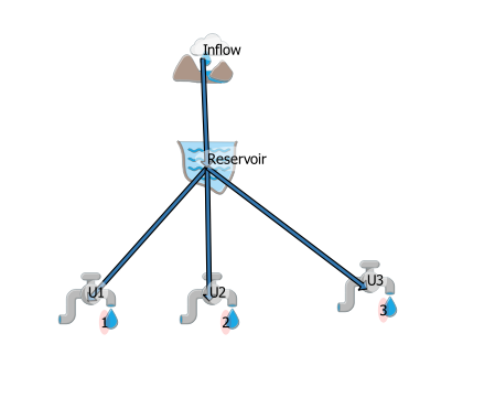
The Single Resource - Multiple Users case does not require a MANAGEMENT node, as it is resolved by priority of the connected USER elements. Common priority USERs share the connected resource deficit. This increases the computational time (due to the fact that the deficit to be shared can not be anticipated a-priori). Thus if more USERs share the same priority and access the same resource, they better be aggregated in a single USER.

Multiple Resources - Single User 

In a Multiple Resources - Single User case, a MANAGEMENT node must be inserted between the resource elements (INFLOW, RESERVOIR, WELLS, ALTERNATIVE RESOURCE) and the USER element.

In the following scheme we may suppose a USER that can access a RESERVOIR, a SPRING and a WELLS field; in the topological scheme, the order of priority is represented by a number next to each USER element

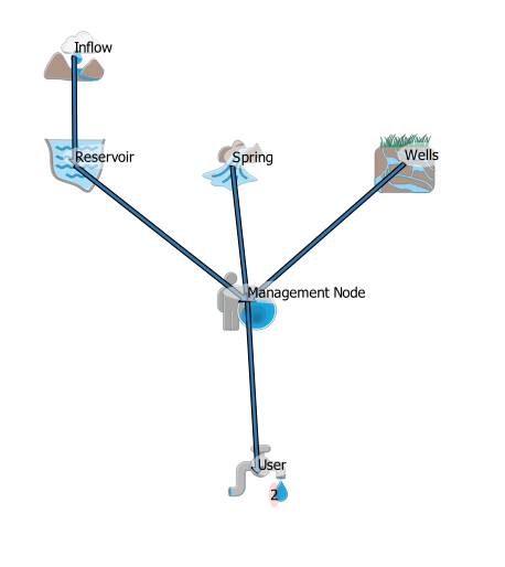
Three built-in approach are currently implemented in the INOPIA MANAGEMENT node:

1. priority management

The USER accesses the resources in priority (e.g. first sends the demand to the RESERVOIR, if not fully supplied then to the SPRING, and finally what’s eventually remains to the WELLS)

1. static allocation management

The USER accesses the resources with predefined monthly allocation ratio (e.g. the user address 0.5 (i.e. 50%) of its demand to the RESERVOIR, 0.3 to the SPRING and 0.2 to the WELLS)

1. dynamic allocation management

The USER accesses the resources with dynamic monthly allocation proportions, depending on the resource availability. The allocation proportions are then estimated by INOPIA management node at each time step during the run, depending on the relation defined by the user between the resource state and the ratio to be used. Such relation, is setable through a parameterization of a generic logistic function, excepted for the last listed resource which will receive all the eventual unadressed demand.

All of these rules are editable through the MANAGEMENT user interface, and further described in the Management node.

Make a connection 

To make a connection, after clicking the icon in the toolbar, left click on the first element and then on the second, and exit the tool with a right click.

Mapping your WSS in INOPIA 

Mapping your WSS in INOPIA is potentially the more complex task, depending on interconnection level. The intention behind INOPIA is being adaptable to each situation. It is unlikely that actually consider/try/describe every possible scheme, but we can suggest some good practices:

1. Identify your ‘MACRO’ resources

If more WELL fields access the same groundwater body, consider to aggregate their maximum pumping rate in a single element. If more SPRINGs come from the same body, and behave similar (i.e. hight correlation among monthly mean discharge) consider to aggregate them. If more INFLOWs end to a common reservoir, consider to aggregate them, and estimate the overall INFLOW (Qin) by level variations (DV) and reservoir discharge observations (Qout) (Qin(t)=DV+Qout(t)) which will include evaporation balance and surface runoff.

1. Identify your ‘MACRO’ USERs

Users sharing same priority, resources and access rules to these resources may be aggregated. This will simplify the scheme, speed up the simulation and simplify their results analysis and interpretation.

1. Split your scheme into “Single Resource - Multiple Users” and “Multiple Resources - Single User” sub schemes

As described in Topology & connections rules identify resources that supply multi-users and user supplied by multiple resources.

1. Contact us

INOPIA is an open source project, developed a GitLab platform. Every potential contributor is welcome. Contribution can range from sharing your issues to joining the GitLab platform as observator or developer of the plugin (Python 3) or the documentation (Sphinx)

Management node 

What is being represented 

The MANAGEMENT node ables to establish the rules for a USER to access multiple resources. A WSS implementation can have more MANAGEMENT nodes.

Built-in model 

Three built-in management rules are currently implemented in the INOPIA MANAGEMENT node, priority management, static allocation managment and dynamic allocation management. Each rule impacts differently the demand allocation scheme as well as associated resources supplied water and deficits. A MANAGEMENT user interface will pop-up once a MANAGEMENT node is connected to a USER and more resources, to able the user to choose and parameterize the rule. The interface will always be accessible through editing, and reset if changes occur in the connections (i.e. removed or added connections)

The selected management rule (and its parameterization) will be applied once the ok button is pressed.

In the following we illustrate the three built-in management rules based on the above example.

1. priority management

The USER accesses the resources in priority. The list of priority can be easily edited by a simple click & drag operation in the connected resources panel.

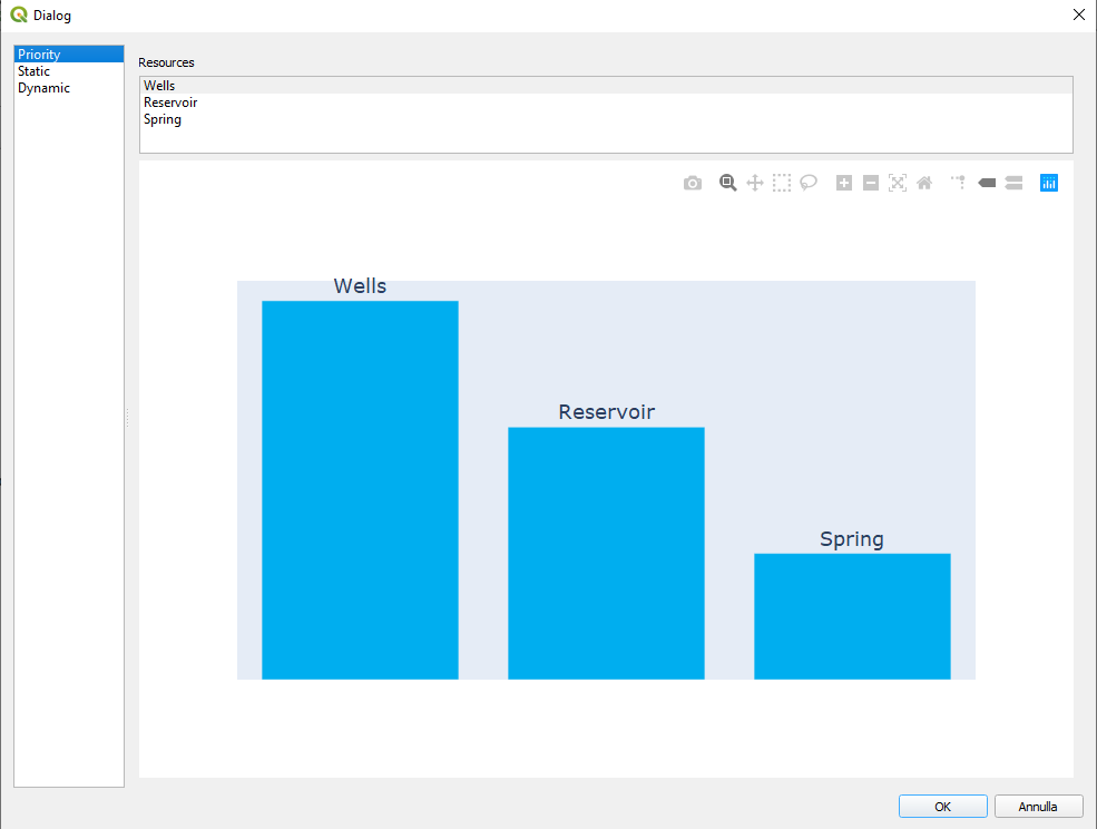
In the example, the USER demand is firstly sent to the WELLS, if not fully supplied to the RESERVOIR, and then to the SPRING. We further illustrate the application of the priority rule for a single month, with a USER demand of 10 Mm ³.

a 10 Mm ³ demand is sent to the WELLS, for which the current maximum pumping rate can supply 2 Mm ³. 8 Mm ³ are still to be supplied to the demand. The WELLS element registers a potential deficit of -8 Mm ³, representing the missing resource necessary to supply all the addressed demand. This deficit is considered potential as this is not an actual deficit for the USER neither for the WSS, as the USER will address the remaining demand to the next resource in the priority list.
remaing 8 Mm ³ demand is sent to the RESERVOIR, for which the current available volume is 5 Mm ³. 3 Mm ³ are still to be supplied to the demand. The RESERVOIR registers a potential deficit of -3 Mm ³, representing the missing resource necessary to supply all the addressed demand. This deficit is considered potential as this is not an actual deficit for the USER neither for the WSS, as the USER will address the remaining demand to the next resource in the priority list.
remaing 3 Mm ³ demand is sent to the SPRING, for which the current discharge can supply 1 Mm ³. The SPRING registers an actual deficit of -2 Mm ³, representing the missing resource necessary to supply all the addressed demand. This deficit is considered actual for the USER and for the WSS, as the USER as no further resource availaible.

The example is limited to a single USER. In case of multi-users, INOPIA will cumulate the USERs and resources deficit and potential deficit following the implemented topology, USER priorities and management rules.

The potential deficit is defined only for priority rule

1. static allocation management

The USER accesses the resources with predifined monthly allocation ratio. The ratio value can be edited in the management user interface. The sum of the ratio for a given month as to be equal to 1. The ratio values can be the same for all months (the checkbox “Change apply to all months” able to fill a full line at once) or be different during the season.

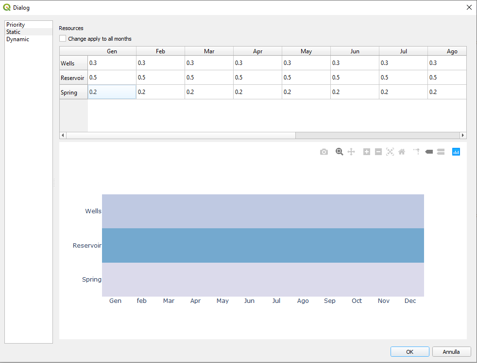
In the example, the ratio is set for all months as 0.3 (i.e. 30%) to the WELLS, 0.5 to the RESERVOIR and 0.2 to the SPRING. We further illustrate the application of the priority rule for a single month, with an USER demand of 10 Mm ³.

30% of the 10 Mm ³ (i.e. 3 Mm ³) demand is sent to the WELLS, for which the current maximum pumping rate can supply 2 Mm ³. The WELLS registers a deficit of -1 Mm ³, representing the missing resource necessary to supply all the addressed sub demand. The USER registers a deficit of -1 Mm ³.
50% of the 10 Mm ³ (i.e. 5 Mm ³) demand is sent to the RESERVOIR, for which the current volume is superior to the demand. The RESERVOIR supplies all the 5 Mm ³ requested. The RESERVOIR registers a null deficit. The USER keeps a deficit of -1 Mm ³.
20% of the 10 Mm ³ (i.e. 2 Mm ³) demand is sent to the SPRING, for which the current discharge can supply 1 Mm ³. The SPRING registers an actual deficit of -1 Mm ³. The USER registers a further deficit of -1 Mm ³, thus a total deficit of -2 Mm ³.

1. dynamic allocation management

The USER accesses the resources with dynamic monthly allocation ratio, depending on the resource availability. The allocation ratio is then estimated by INOPIA management node at each time step during the run, depending on the relation defined by the user between the resource state and the ratio to be used. Such relation is setable through a parametrization of a generic logistic function, except for the last listed resource which will receive all the eventual unadressed demand. The ranking of the resource list can be changed by a simple click & drag operation in the connected resources panel. The logistic function has been chosen as it is able to reproduce both a stepwise (highly non-linear) and a smooth (close to linear) decision process. Six parameters define the logistic function, linking the resource state to the demand ratio.

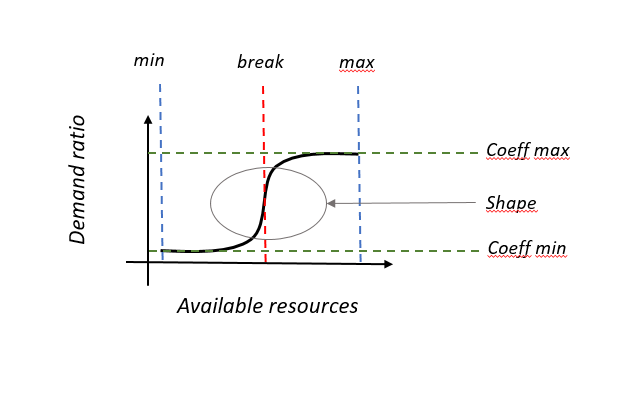
Four parameters define the range of the function:
-“min” and “max” are the minimum and maximum resource value along which the logistic is defined. The unit to be considered depends on the type of resource.

-“Coeffmin” and “Coeffmax” are the minimum and maximum ratio values.
Two parameters define the shape of the function:
-“break” defines the resource value at which a decision is taken (with a ratio tending toward “coeffmin” if the resource state is less than the “break” value and a ratio tending toward “coeffmax” if the resource state is more than the “break” value)

-“shape” modifies the shape of the resulting logistic function, from a sharp change (toward “coeffmin” and “coeffmax” at “break”) to a smooth change, depending on the value, as illustrated in the following example.

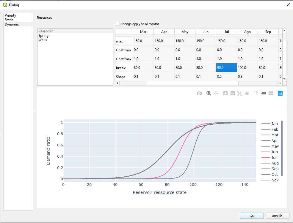
In the example, the WELLS is firstly addressed, secondly the RESERVOIR, and lastly the remaining demand is addressed to the SPRING.

The WELLS state (Q disp) for the current month, considering the logistic parametrization of the considered month, leads to a ratio of 0.2. 20% of the 10 Mm ³ (i.e. 2 Mm ³) demand is sent to the WELLS, for which the current maximum pumping rate can supply 2 Mm ³. The WELLS and the USER register a null deficit.
The RESERVOIR state (V disp) for the current month, considering the logistic parametrization of the considered month, leads to a ratio of 0.5. 50% of the remaining 8 Mm ³ (i.e. 4 Mm ³) demand is sent to the RESERVOIR, the current available volume is 3 Mm ³. The RESERVOIR and the USER register a deficit of -1 Mm ³.
All the remaining demand (10-2-4)= 4 Mm ³ demand is sent to the SPRING, for which the current discharge can supply 2 Mm ³. The SPRING registers a deficit of -2 Mm ³. The USER registers a further deficit of -2 Mm ³, thus a total deficit of -3 Mm ³.

Run 

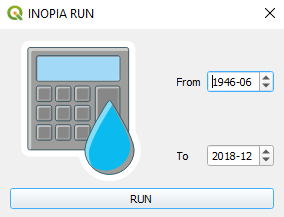
Run hindcast 

The Hincast run is the central INOPIA brain. It calculates the monthly mass balance of the implemented system.

A simple UI ables the user to select the timeline to be simulated, proposing by default the maximum timeline for which all necessary data are available (also considering the scale of SPI calibrated for SPRING and INFLOW elements).

Hincast run should be able to adapt to any scheme that follows the “Topology & connections rules” using the data supplied to each connected element through their excel templates. The mass balance is done both at element and water supply level, each element storing its own mass balance.

Hindcast run provides a direct way to test your implemented WSS against observations if they are available. INOPIA plot built-in tools provide assessment of SPRING and INFLOW discharge estimation as well as visual comparison with RESERVOIR observed lake level variation if supplied. The built-in export tools able to make any possible kind of assessment of any element of the INOPIA mass balance depending on the available observation, to adapt to any needs.

Moreover, hindcast run can be easily used for many other purpose as

-management scenarios by adding/editing management elements

-infrastrucure scenarios by adding/editing resources elements and/or connections

-demands scenarios by adding/editing user elements

-climate scenarios by providing precipitation scenarios data to INFLOW and SPRING templates

all of these scenarios can easily be combined, making INOPIA a versatile DDS.

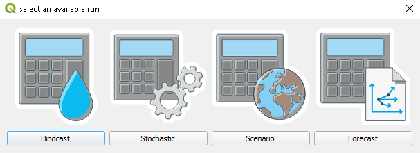
Other runs have been pre-implemented to simplify the use of the hindcast run for specific demands, all based the same algorithm. Their use will become available after a first hindcast run.

Run stochastic 

“what if I had 500 years of mass balance data on my WSS running as it is under a stationary climate to do some better statistics?”

You may want to use INOPIA to supply robust statistics on your WSS (for built-in drought indexes estimation and early warning DSS or any other needs through the export tools).

Robust statistics on deficit events usually need significantly more data than what supplied to the hindcast (tipically few decades), as usually the WSS and the water needs adapt to each other for a given territory while precipitation drought are by definition rare on a stationary climate baseline.

So you may want to supply INOPIA with centuries of weather generated data to answer the demand “what if I had 500 years of mass balance data on my WSS running as it is under a stazionary climate to do some better statistics?”. The run stochastic will do that for you.

It will generate 500 years of random precipitation data following the autocorrelation pattern learned from the Hindcast precipitation anomalies and will apply the hindcast calibration of the discharge built-in model. A description of the weather generator and its implementation can be found in Romano et al., 2017.

Run Scenario 

“How does my water supply system behave under climate change scenarios? How can I adapt ?”

You may want to use INOPIA to support climate change adaptation.

Precipitation drought is by definition rare on a stationary climate baseline. Differently, the ongoing climate change affects precipitation variability including seasonality, large scale periodicity as well as frequencies and intensity of extreme anomalies.

“Climate models are one of the primary means for scientists to understand how the climate has changed in the past and may change in the future. These models simulate the physics, chemistry and biology of the atmosphere, land and oceans in great detail, and require some of the largest supercomputers in the world to generate their climate projections. Climate models are constantly being updated, as different modelling groups around the world incorporate higher spatial resolution, new physical processes and biogeochemical cycles. These modelling groups coordinate their updates around the schedule of the Intergovernmental Panel on Climate Change (IPCC) assessment reports, releasing a set of model results.” https://www.carbonbrief.org/cmip6-the-next-generation-of-climate-models-explained/

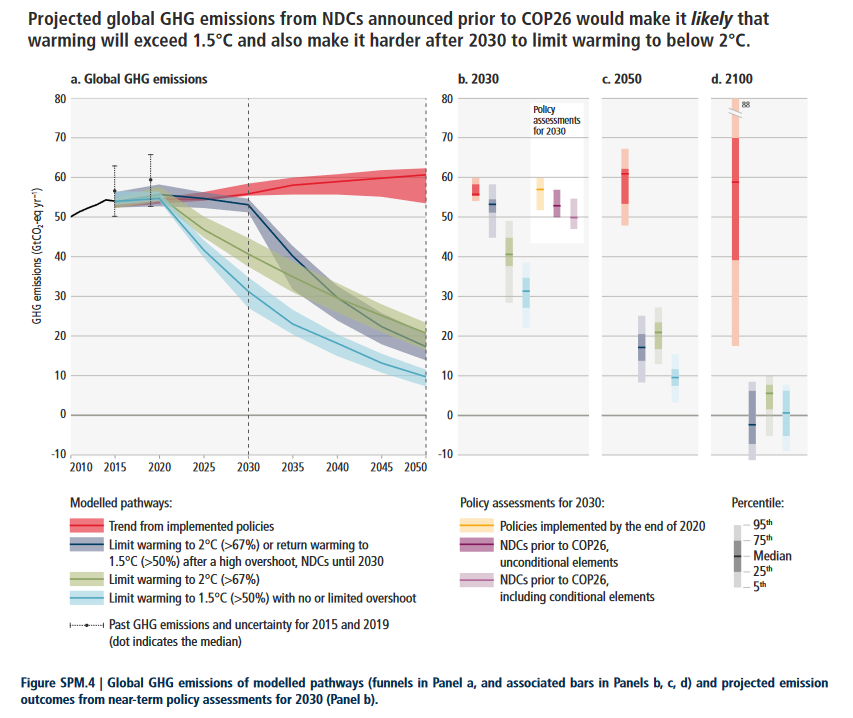
(figure from https://www.ipcc.ch/report/ar6/wg3/downloads/report/IPCC_AR6_WGIII_SPM.pdf)

So you may want to supply INOPIA with climate models scenarios using hindcast parametrization to answer the demand “How does my water supply system behave under climate change scenarios? How can I adapt ?”. The run scenario will do that for you.

It will ask you to provide a precipitation scenario for each INFLOW and SPRING connected elements containing the precipitation climate scenarios you want to test. As run scenarios will use the hindcast parametrization, the precipitation scenarios supplied should be downscaled on the stations used in each element in the hindcast, so that their quantiles follows the same distribution (this can be done with simple quantile mapping for example, e.g. Guyennon et al., 2013).

As many climate models, emission scenarios, statistical downscaling technics exist, constantly updated, the selection of monthly precipitation climate model/scenarios/dowscaling is up to the user and supplied to INOPIA through the simple precipitation template file (link )

The Run scenario can be combined with management, infrastructure and demands scenarios by editing the implemented WSS before running the climate scenario.

Run Forecast 

“How will my water supply system behave in the coming months ?”

You may want to use INOPIA to support short-term (one to six months) decision support based on seasonal forecast.

So you may want to supply INOPIA with seasonal precipitation scenarios based on probability of occurence of wet or dry situations in the coming months to answer the question “How will my water supply system behave in the coming months ?”. Such scenarios may be based on the on-going effort on seasonal climate tendency modeling and often express in expected anomalies (e.g. wet, normal, dry) or on anomalies classification as for example that of the European Drought Observatory (EDO)

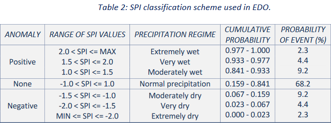
(Table from https://edo.jrc.ec.europa.eu/documents/factsheets/factsheet_spi.pdf)

It means that you should supply INOPIA with next 6 months expected precipitation for each stations used for each INFLOW and SPRING connected elements based on an expected anomaly scenario. The run forecast will do that for you.

It will simply ask you to provide a common precipitation expected anomaly [-3 3] to the implemented water supply system and run a 6 months forward simulation.

Edit tool 

Applied on Resources element 

The EDIT tool applied to the Resources elements allows the user to select new input files for the selected resource.

In case of editing of a resource element, for example in this case an INFLOW element, after confirming to start editing, the user will be asked to supply a new precipitation file and discharge file according to the templates ( Input template)

Previous run will have to be recalculated to take the change into account.

*Tip & tricks : ‘You can use edit on INFLOW and SPRING elements to update hindcast (and thus forecast) simulations with last available monthly precipitation’

Applied on Users element 

The EDIT tool applied to the Users elements allows the user to change the priority level assigned during the creation of the USER element.

Previous run will have to be recalculated to take the change into account.

Applied on Management element 

The EDIT tool applied to the Management element allows the user to change the selected management rule and its parametrization.

Previous run will have to be recalculated to take the change into account.

Built-in plotting tool 

INOPIA proposes 3 kinds of integrating built-in plotting tool to support the user in assessing his WSS.

A simple user interface ables to choose the run to be plotted among those available.

1. plot time series applied to each single element (except the management node)
1. plot diagnostic, applied to each single element (except the management node)
1. plot diagnostic, applied to the overall WSS

Each plot is described in the following.

Plot element time series 

Plot time series applied to each single element and each run (except the management node). After selecting the “plot element time series” icon, the user clicks on the element to be displayed, and selects an available run to generate the figure.

The upper panels of the figure is dedicated to the element input information, independently of the selected run. The lower panel plots the monthly mass balance variables of the considered element and run expressed in Mm ³. The user can interactively select the variables to be displayed.

The plot time series is illustrated in the following with two examples from the tutorial.

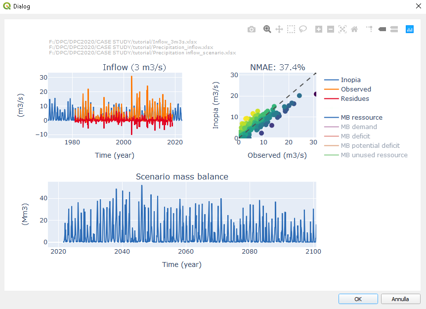
_images/plot_ts_inflow_sce.PNG — *Example of plot element time series applied to the tutorial INFLOW scenario run*

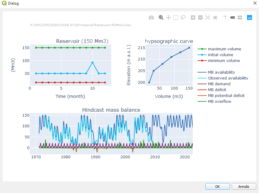
_images/plot_ts_reservoir_hin.png — *Example of plot element time series applied to the tutorial RESERVOIR hindcast run*

Tip & tricks: It also applies to new element without available run which may be useful to monitor INFLOW and SPRING built-in model results

Plot element diagnostic 

Plot element diagnostic applied to each single element and each run (except the management node). After selecting the “plot element diagnostic” icon, the user clicks on the element to be displayed, and selects an available run to generate the figure.

The left panel of the figure is dedicated to the monthly mean value of the mass balance variables of the considered element expressed in Mm ³. The user can interactively select the variables to be displayed, as well as the period (within the selected run) and month to be considered.

The upper right panel of the figure is dedicated to the risk of deficit of the element, in terms of probability of occurrence (reliability), duration (resiliency) and intensity (vulnerability) indexes following Romano et al., 2017. The stochastic run has been designed to produce more robust estimation of the drought indexes. The user can interactively select the period (within the selected run) and the month to be considered for the RRV indexes estimations.

The lower right panel of the figure is dedicated to the inter-element flux, considering all elements connected to the selected one. The user can interactively select the flux to be considered among allocated water, deficit and potential deficit as well as the period (within the selected run) and the month to be considered for the Sankey diagram elaboration.

The plot element diagnostic is illustrated in the following with two examples from the tutorial.

_images/plot_diag_user.png — *Example of plot element diagnostic applied to the tutorial USER scenario*

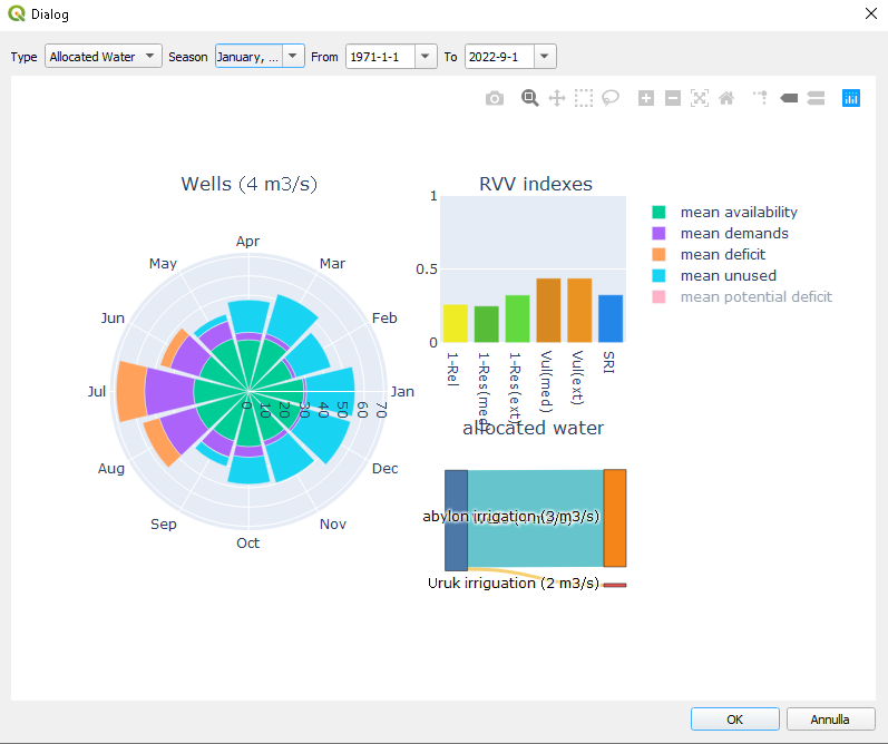
_images/plot_diag_well.png — *Example of plot element diagnostic applied to the tutorial WELLS hindcast*

Plot WSS diagnostic 

Plot WSS diagnostic applied to the all implemented elements and each run (except the management node). After selecting the “plot element diagnostic” icon, the user selects an available run to generate the figure.

The left panel of the figure is dedicated to the inter-element flux, considering all elements connected to the selected one. The user can interactively select the flux to be considered among allocated water, deficit and potential deficit as well as the period (within the selected run) and the month to be considered for the Sankey diagram elaboration.

The upper right panel of the figure is dedicated to the monthly mean value of the mass balance variables of the WSS expressed in Mm ³. The user can interactively select the variables to be displayed, as well as the period (within the selected run) and the month to be considered.

The lower right panel of the figure is dedicated to the risk of deficit of the WSS, in terms of probability of occurrence (reliability), duration (resiliency) and intensity (vulnerability) indexes following Romano et al., 2017. The stochastic run has been designed to produce more robust estimation of the drought indexes. The user can interactively select the period (within the selected run) and the month to be considered for the indexes estimations.

The plot element diagnostic is illustrated in the following with two examples from the tutorial.

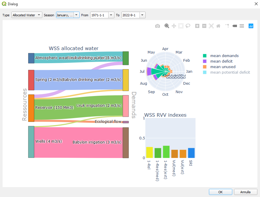
_images/plot_all_hin.png — *Example of plot WSS diagnostic applied to the tutorial hindcast with Sankey diagram of allocated water.*

_images/plot_all_def_sce.png — *Example of plot WSS diagnostic applied to the tutorial scenario with Sankey diagram of deficit.*

Early Warning tool 

Early warning is an INOPIA built-in tool helping the user in early warning decision support. It is based on the relation between observed precipitation anomalies and simulated deficit, as a proxy to the relation between meteorological drought and relative impact on the water safety. It relies on the fact that for a given month of the year, the occurence and intensity of a possible deficit (as a measure of the impact on the water safety) during the coming months can partially be predicted based on the precipitation anomalies of the previous months, based on the experience learned. The early warning approach and methods is fully described in Romano et al., 2018

The early warning tool applies in the same way to hindcast, stochastic and scenarios run, but gives more robust results with the stochastic simulation. After selecting the element, a simple user interface ables to choose the run to be plotted among those available.

Early warning currently applies to RESERVOIR and SPRING elements.

RESERVOIR early warning 

After selecting the “early warning” icon, the user clicks on the considered RESERVOIR, and selects an available run to generate the figure.

In the upper menu, the user selects:

the reference month (when to take a decision). In the proposed example the selected reference month is April.
the SPI aggregation scale (previous precipitation). In the proposed example the selected reference months are 6 months.
the deficit aggregation scale (future deficit). In the proposed example the selected reference months are 5 months.

following the example, the early warning demand is:

“considering the precipitation anomalies from November to April (i.e. April SPI6) how well can I predict the occurence and intensity of next May to September deficit?”

The upper left panel presents the relation between the SPI predictor (the reference month precipitation anomaly cumulated on the selected aggregation scale (April SPI6 following the example) and the possible deficit during the next deficit aggregation scale months (next 5 months, May to September, following the example). On the hypotesis of a fairly linear relation between the SPI predictor and future deficit, an SPI alarm level can be estimated as the value at which the linear regression of the non-null cumulated deficit intersects the SPI predictor axis. In case the estimated SPI alarm is positive (which indicates a structural deficit condition of the RESERVOIR), the SPI alarm is set to 0.

Moreover, when applied to a storage capacity, knowing the current state of the resource can further support the prediction. The upper right panel presents the relation between the volume stored at the reference month (April following the example) and the possible deficit during the next deficit aggregation scale months (next 5 months, May to September, following the example). Similarly to the SPI alarm , a Volume alarm can be estimated as the Volume value at which the linear regression of the non-null cumulated deficit intersects the Volume axis. In case the optional hypsographic input sheet is present, the volume alarm can be expressed as level alarm in m a.s.l.

The lower panels of the figure are dedicated to the lesson learned from the previous relation.

The early warning demand with associated estimated SPI and volume alarms are summarized on the left, and the resulting early warning model is tested: a deficit is predicted if the SPI predictor is less than the estimated SPI alarm and the reference month volume is less than the estimated volume alarm. Each month of the considered run is then classified into:

True Positive (TP) : a deficit has been predicted and actually occured
False Positive (FP): a deficit has been predicted but does not actually occured
True Negative (TN) : no deficit has been predicted and no deficit actually occured
False Negative (FN) : no deficit has been predicted but a deficit actually occured

the classification is reported in the confusion matrix on the bottom right panel.

Finally the early warning model performance can be evaluated in term of:

The True Positive Rate (TPR), defined as the ratio between the True Positive cases (TP) and the actual positive cases (TP+FN): TPR=TP/(TP+FN)
The False Positive Rate (FPR), defined as the ratio between the False Positive cases (FP) and the actual negative cases (TN+FP): TPR=FP/(TN+TP)

both the TPR and FPR are defined between [0-1].

The more the early warning model tends toward a maximum (->1) True Positive Rate and a minimum (->0) False Positive Rate the more robust it is. The True Positive Rate and False Positive Rate are reported on the lower left panel.

The RESERVOIR early warning is illustrated in the following with two examples from the tutorial.

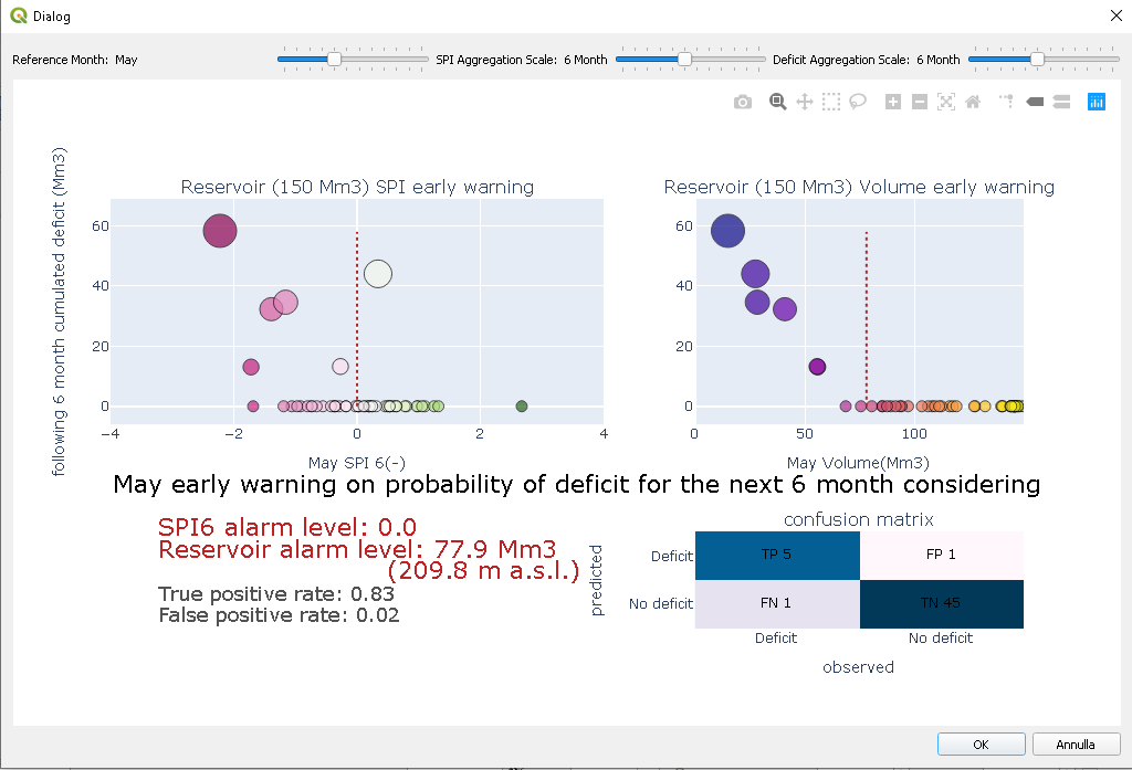
_images/ew_reservoir_hin.png — *Example of plot EW applied to the tutorial RESERVOIR hindcast run.*

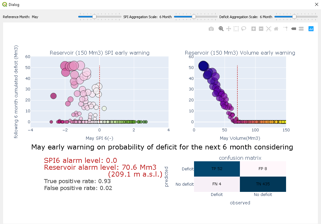
_images/ew_reservoir_sto.png — *Example of plot EW applied to the tutorial RESERVOIR stochastic run.*

The early warning plot will automatically update as any of the user parameter change. This ables to test the response of the RESERVOIR to different combination of scales for a given month, and identifies the best EW capacity for a given WSS configuration.

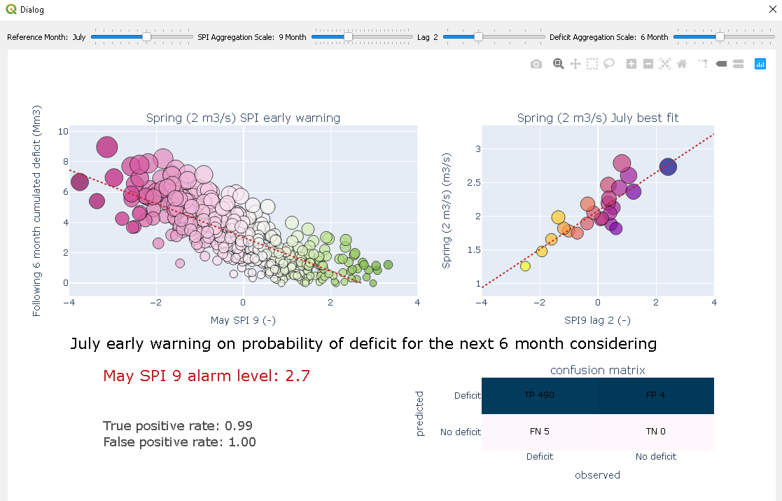
SPRING early warning 

After selecting the “early warning” icon, the user clicks on the considered SPRING, and selects an available run to generate the figure.

In the upper menu, the user selects:

the reference month (when to take a decision). In the proposed example the selected reference month is July.
the SPI aggregation scale (previous precipitation). In the proposed example the selected reference months are 9 months.
the SPI lag (mean infiltration delay). In the proposed example the selected reference months are 2 months.
the deficit aggregation scale (future deficit). In the proposed example the selected reference months are 6 months.

Following the example, the early warning demand is

“considering the precipitation anomalies from September to May (i.e. May SPI9) how well can I predict the occurence and intensity of next August to January deficit?”

The upper left panel presents the relation between SPI predictor (the reference month precipitation anomaly, considering the lag, cumulated on the selected aggregation scale, May SPI9 following the example) and possible deficit during the next deficit aggregation scale months (next 6 months, August to January, following the example). On the hypotesis of a fairly linear relation between the SPI predictor and future deficit, an SPI alarm level can be estimated as the value at which the linear regression of the non-null cumulated deficit intersects the SPI predictor axis.

The upper right panel presents the best relation found during the calibration of the SPRING built-in model for the reference month.

The lower panels of the figure are dedicated to the lesson learned from the previous relation.

The early warning demand with associated estimated SPI and volume alarms are summarized on the left, and the resulting early warning model is tested: a deficit is predicted if the selected SPI predictor value is less than the estimated SPI alarm. Each month of the considered run is then classified into:

True Positive (TP) : a deficit has been predicted and actually occured
False Positive (FP): a deficit has been predicted but does not actually occured
True Negative (TN) : no deficit has been predicted and no deficit actually occured
False Negative (FN) : no deficit has been predicted but a deficit actually occured

the classification is reported in the confusion matrix on the bottom right panel.

Finally the early warning model performance can be evaluated in term of:

The True Positive Rate (TPR), defined as the ratio between the True Positive cases (TP) and the actual positive cases (TP+FN): TPR=TP/(TP+FN)
The False Positive Rate (FPR), defined as the ratio between the False Positive cases (FP) and the actual negative cases (TN+FP): TPR=FP/(TN+TP)

both the TPR and FPR are defined between [0-1].

The SPRING early warning is illustrated in the following with two examples from the tutorial.

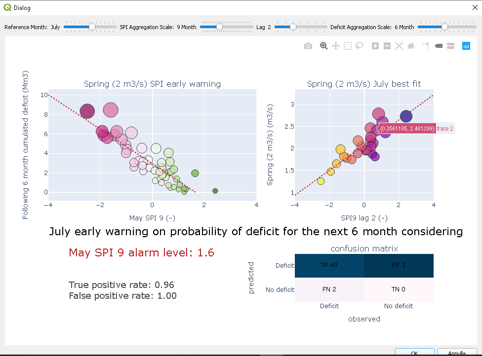
_images/ew_spring_hin.png — *Example of plot EW applied to the tutorial SPRING hindcast run.*

_images/ew_spring_sto.png — *Example of plot EW applied to the tutorial SPRING stochastic run.*

Exporting 

The export tool ables exporting in xlsx format times series of a single element, as well as mass balance of the entire WSS, for a selected RUN. This ables expert user to build his own grafics and analysis using the same data as INOPIA.

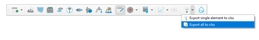
A simple user interface ables to choose the run to be ploted among those available.

Tip & tricks : Export is available on single element even without any connection nor run executed. This ables to use and export the built-in model results of INFLOW and SPRING as well as calcultaed SPI values.