Quick start

Following this quick start you can install QGIS (if necessary) and INOPIA, learn how to manage an INOPIA project within QGIS and create a first water supply system exploring most of the INOPIA functionalities thanks of the proposed tutorial case study.

Download & install QGIS & INOPIA

STEP 1 - Install QGIS updated to Python 3

QGIS is a leading professional GIS application that is built on top of and proud to be itself Free and Open Source Software

QGIS can be downloaded and installed from

https://www.qgis.org/en/site/forusers/download.html

we suggest to install the Long term release

minimum version 3.22

STEP 2 - Install INOPIA plugin

Once installed QGIS, INOPIA can be installed as a plugin in two steps:

1- to download INOPIA 3.0 please contact info-inopia@irsa.cnr.it

2- open QGIS, click on Plugins –> Manage and Install Plugins –> install from zip , point to the download file (inopia.zip) and click on Install plugin.

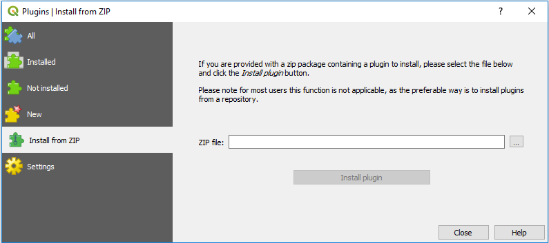
Note

INOPIA may install the python libraries statsmodels and openpyxl, not available with the standard installation of QGIS. In such case, close and restart QGIS to make INOPIA available.

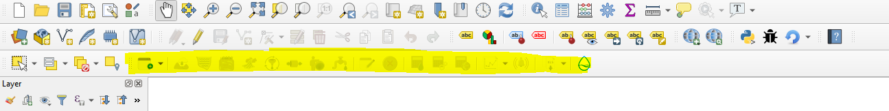
The INOPIA toolbar is now available, ready to create your first INOPIA project, within an existing or new QGIS project.

more information on QGIS plugins can be found here

https://www.qgistutorials.com/en/docs/3/using_plugins.html

Managing your INOPIA project in QGIS

INOPIA is a toolbar plugin to be used in a QGIS project. INOPIA works on his own files, creating/updating associated INOPIA layers into a GIS. This means that an INOPIA project can be created into a new or existing GIS project, and be loaded/edited later in the same or other GIS projects.

Note

INOPIA WILL SAVE AUTOMATICALLY ALL CHANGES INTO THE INOPIA FILES.

This is to make sure that what you see (layers) perfectly corresponds to what is inside the project binary file (.inopia). No undo function is available, you will need to use the INOPIA built-in EDIT and CANCEL function. The SAVEAS function can be useful to work on a project copy or to create backup.

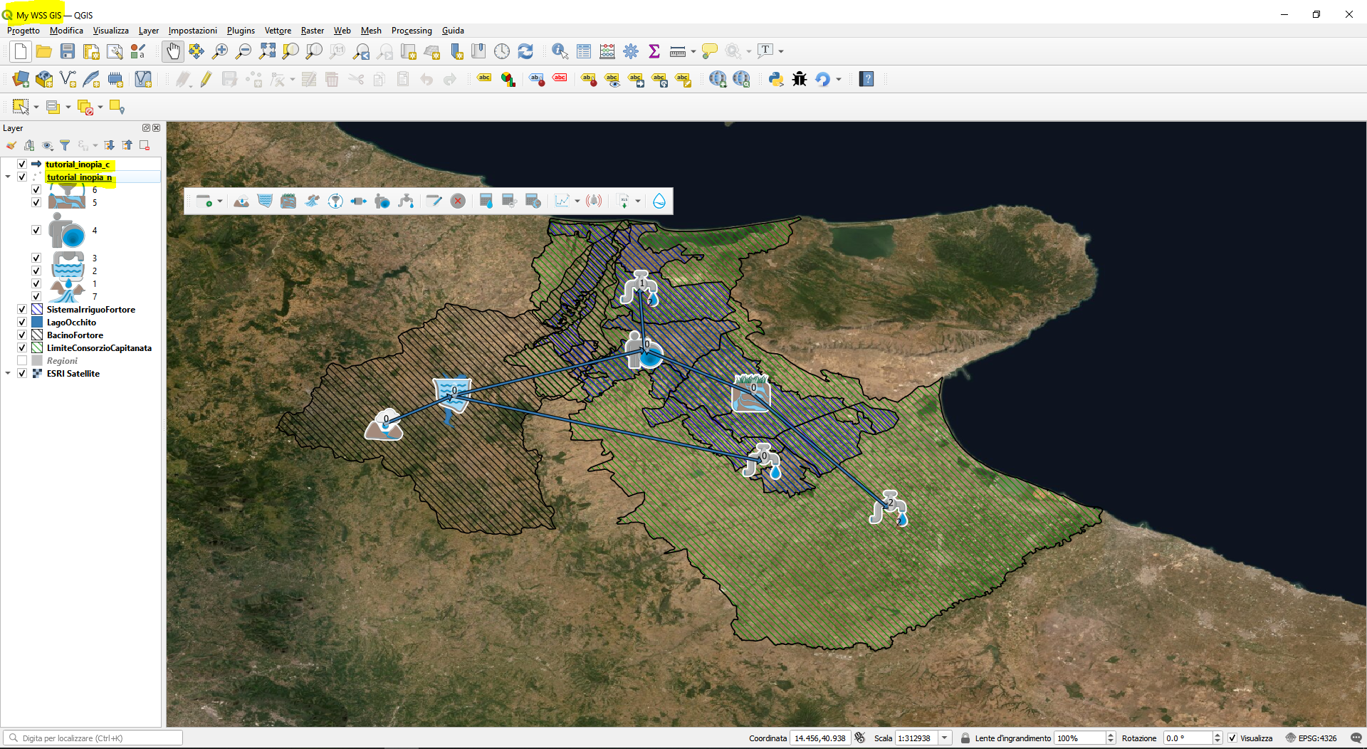
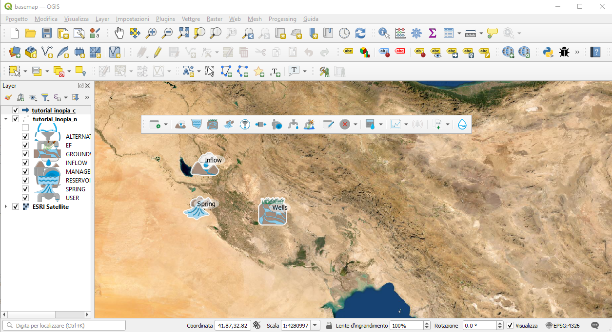
In the following example, the QGIS project is “My WSS GIS”, containing more layers of previous works, while the INOPIA project is “tutorial”, with its own two layers, tutorial_inopia_c and tutorial_inopia_n. These layer are created and updated automatically by INOPIA, and should not be renamed nor edited manually.

INOPIA will created/load/save 2 files associated to the INOPIA project (a geopackage containing inopia layers and a binary file). The user does not have to care about these files, as they are autonomously and automatically managed by INOPIA. None of these files should be manually edited.

To share an INOPIA project, only those two files need to be sent.

In the following the new/load/saveas icons from the INOPIA toolbar are shorly described

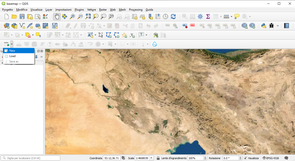
New

New Icon

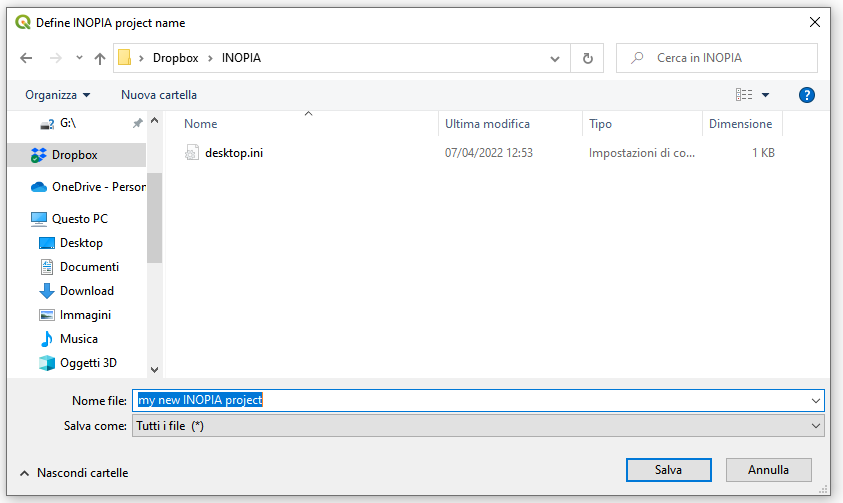
The New icon ables to create a new INOPIA project into your QGIS project. More INOPIA projects can be created into the same QGIS project. Once clicking on New icon, you will be invited to choose a path and an INOPIA project name.

Load

Load Icon

The Load icon ables lo load a previous INOPIA project into your QGIS project. Only one INOPIA project can be loaded at time. Once clicking on Load icon, you will be invited to choose and load a previous INOPIA project

Save as

saveas icon

The Saveas icon ables to save the current INOPIA project with a new project name. Once clicking on Saveas icon, you will be invited to choose a new path and an INOPIA project name. The new project will be automatically loaded into your QGIS project. This able us to safely work on scenarios/editing etc.. starting from an existing project, while the previous “current” project is safe, and can be reloaded later.

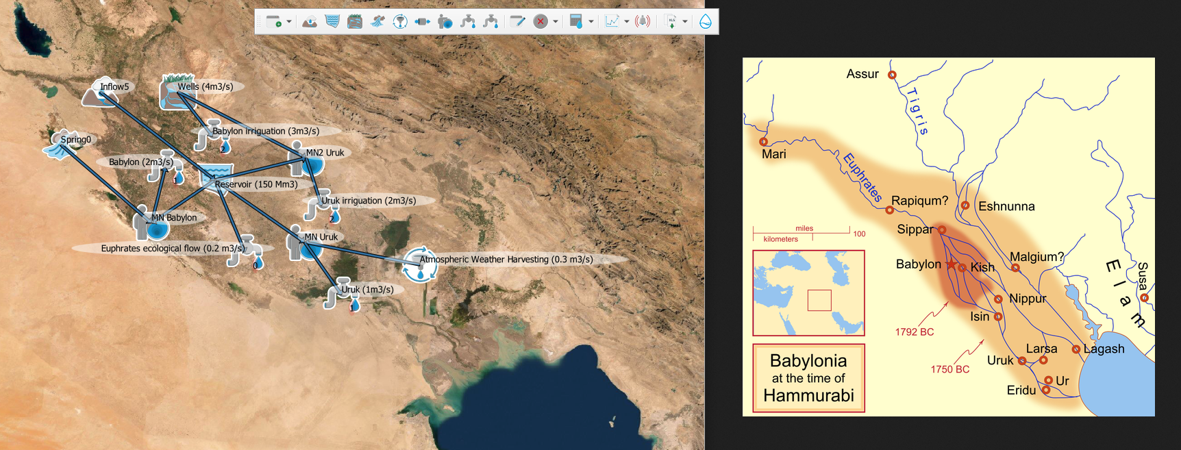
Create your first WSS (Tutorial)

The proposed tutorial is only didactic, dedicated to explore the INOPIA elements and functions.

The storyboard, scheme and numbers provided in the tutorial are a deep fantasist re-interpretation of the early beginning of irrigation for a ludic introduction to INOPIA and are not aimed at reproducing any historical reality.

To follow the proposed tutorial step by step, the complete dataset is available at the following link including input data files and the final result of the INOPIA project.

Chapter #1 The resources

Open QGIS, with INOPIA installed (cf Download & install QGIS & INOPIA).

You can both start from an empty QGIS project or load a previous one. In the tutorial dataset you can find and load a QGIS project (basemap.qgz) with the ‘ESRI satellite’ as basemap. In the following we load QGIS basemap.qgz project.

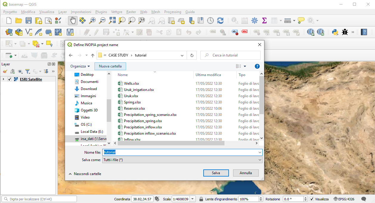
To begin with a new INOPIA project, we select icon from the inopia toolbar.

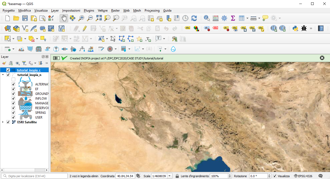
You will be invited to indicate a new INOPIA project name. Note that the INOPIA design ables you to load more INOPIA projects into a QGIS project (only the last INOPIA loaded project is active). Moreover an INOPIA project can be loaded in any QGIS project. We indicate “tutorial” as INOPIA project name.

You have just created your first INOPIA project. Now the elements in the INOPIA toolbar became available. Two layers have been added to the QGIS project. These layers are created and managed by INOPIA. Do not edit them manually. They are both stored in the geopackage “tutorial.gpkg”. A binary file “tutorial.inopia” has also been created, storing the binary data from the INOPIA project. These two files contain all the information of your project, and can easily be shared with other users having INOPIA installed.

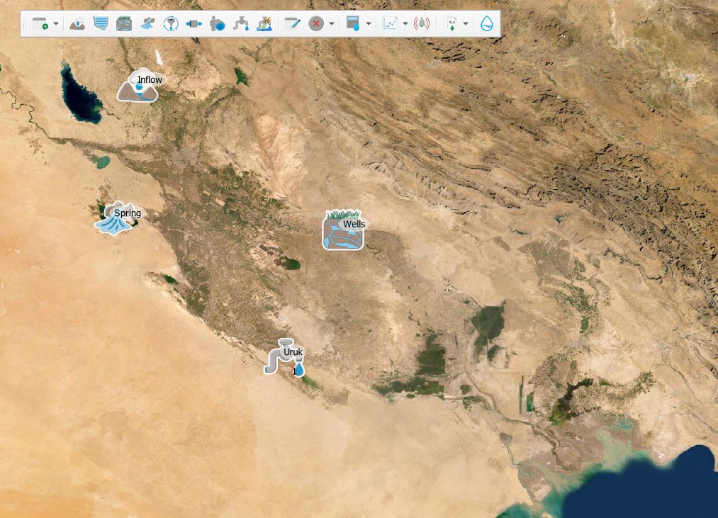
In this first chapter of the tutorial, we will set three resources, an INFLOW, a SPRING and a WELLS field.

To add an INFLOW resource first, we click on the icon and then to the location on the map (we select roughly 44° east and 34° north). INOPIA does not consider the coordinates of each element in its algorithms, the positioning being for INOPIA a visual support to build the topological scheme. INOPIA will pop up a windows asking to set the element name to be used in the INOPIA project to identify the element. Do not give the same name to more elements, as the element name is a primary key for INOPIA. Further two windows will pop-up to ask firstly a precipitation file, and secondly an inflow file to feed the new element. We indicate as element name “inflow”, as precipitation file “Precipitation_inflow.xlsx” and as inflow file “inflow.xlsx” (provided in the tutorial dataset)

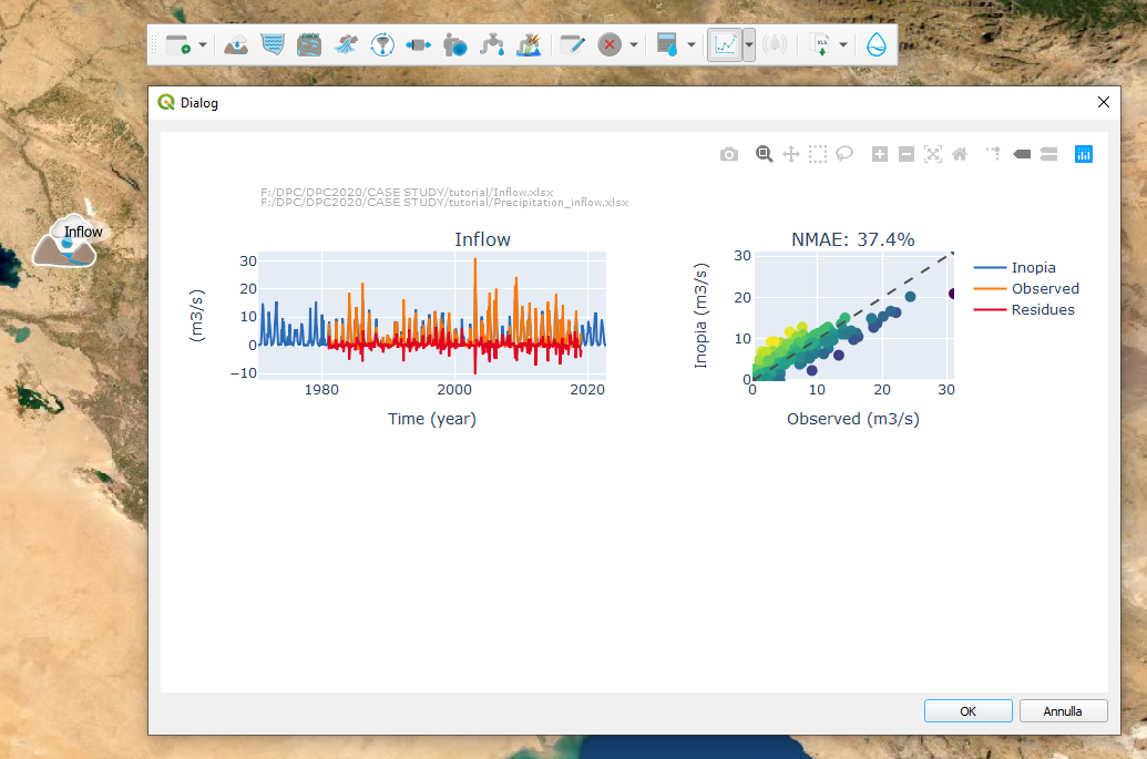
You have just created your first INOPIA element. Now you can monitor the new INFLOW element using the icon. Click on the plot icon, and then on the INFLOW element.

The SPRING resource creation follows the same steps as the INFLOW. Click on the icon and then to the location on the map. We indicate as element name “spring”, as precipitation file “Precipitation_spring.xlsx” and as spring file “spring.xlsx” (provided in the tutorial dataset). Similarly, the SPRING element can be monitored using the plot icon after being created. Finally, similarly to INFLOW and SPRING, we add a resource. A single input file is needed for the WELLS element. We indicates as element name “wells” and as wells file “Wells.xlsx” (provided in the tutorial dataset).

You should end up with the three resources implemented in your tutorial INOPIA project.

You can export the element dataset using the icon. Click on export icon and then on the element to export. Finally indicate a place and a filename to export the data. This gives the possibility to export the results of INOPIA built-in models for the inflow and spring elements

Chapter #2 Uruk

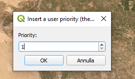
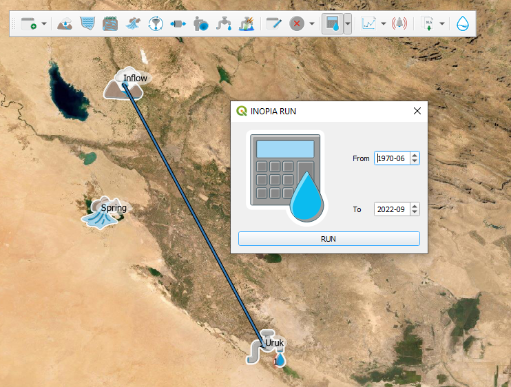
Once set the resources, we add the demands. In our tutorial, we propose to set a drinking water and an irrigation demands for the cities of Uruk and Babylon. To set a USER demand, click on the icon and then indicate the position on the map. INOPIA will pop up a windows asking to set the element name (we set “Uruk”) and a priority. The USER priority is an integer between 1 and 10, 1 being the highest priority and 10 the lowest. Since the USER is a drinking water demand, we set a priority equal to 1. After setting the priority, a window will pop-up to ask for a USER input file. We indicate the tutorial file Uruk.xlsx.

Now we can supply the Uruk drinking water demand with the INFLOW resource. To do so, we click on the icon, then first on the INFLOW element, then on the Uruk USER element (as the water flows from the INFLOW to the USER) and finally right click to finalize the connection construction.

You have just created your first INOPIA connection. Having connected a resource to a demand, you can now run a first mass balance, by clicking on the . The hincast run user interface will pop-up to indicate the first and the last month to be considered. The user interface is pre-compiled with the first and last available data for simulation (in the tutorial, from June 1970 to September 2022, as June 1970 is the first month of the precipitation file supplied, having a value for SPI6, used in the inflow built-in model)

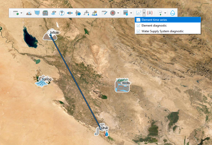
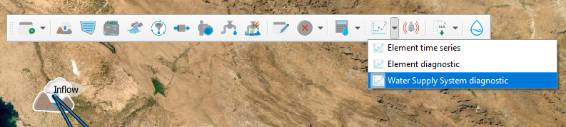
Now a hindcast run is available for the connected elements. You can click on and indicate the INFLOW or the Uruk USER. Three built-in plot functions are now available. First two (“element time series” and “element diagnostic”) apply to an element, while the third (“Water Supply System diagnostic”) apply to all the connected elements.

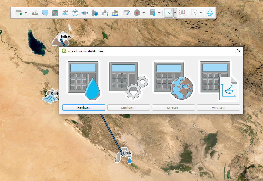
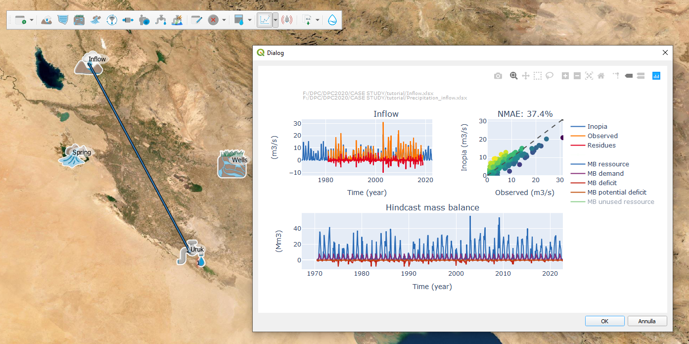
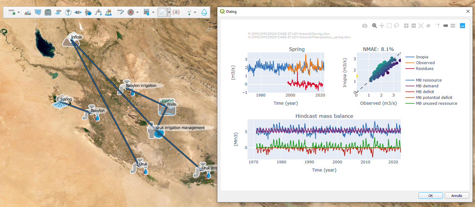
Here we select to plot “element time series” and apply it to the INFLOW element. A user interface will pop-up to let you to indicate the run to be plotted (here the only hindcast is available)

The selected run mass balance for the selected element (inflow hindcast in the example) is shown on the lower panel.

We now add the Uruk irrigation demand, clicking on the icon and then to the location on the map. We call the USER “Uruk irrigation”, set a priority equal to 2, indicate the tutorial input file “Uruk_irrigation.xlsx’ and connect the Uruk irrigation to the same INFLOW resource.

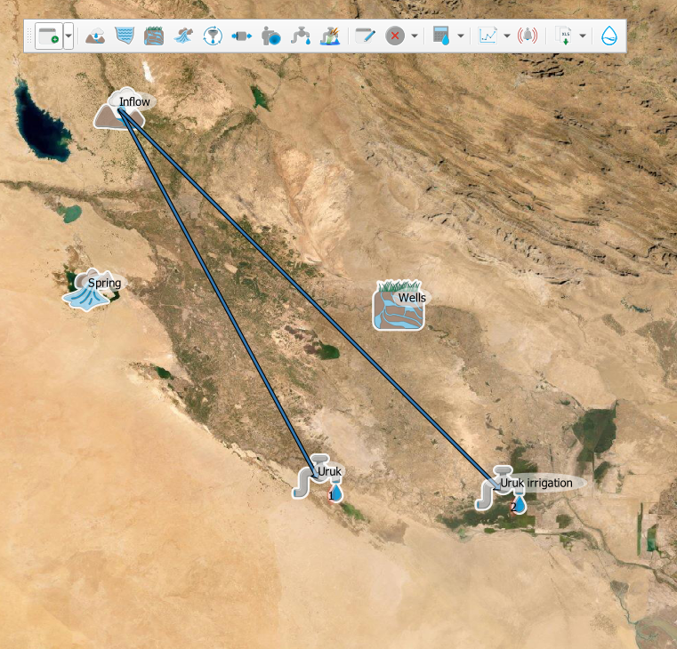
This is the case of a simple mono resource - multi user sub scheme introducing allocation by USER priority: the irrigation demand with priority = 2 will be supplied after the drinking water demand with priority = 1.

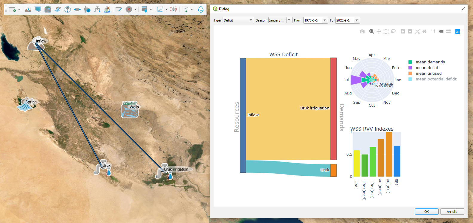
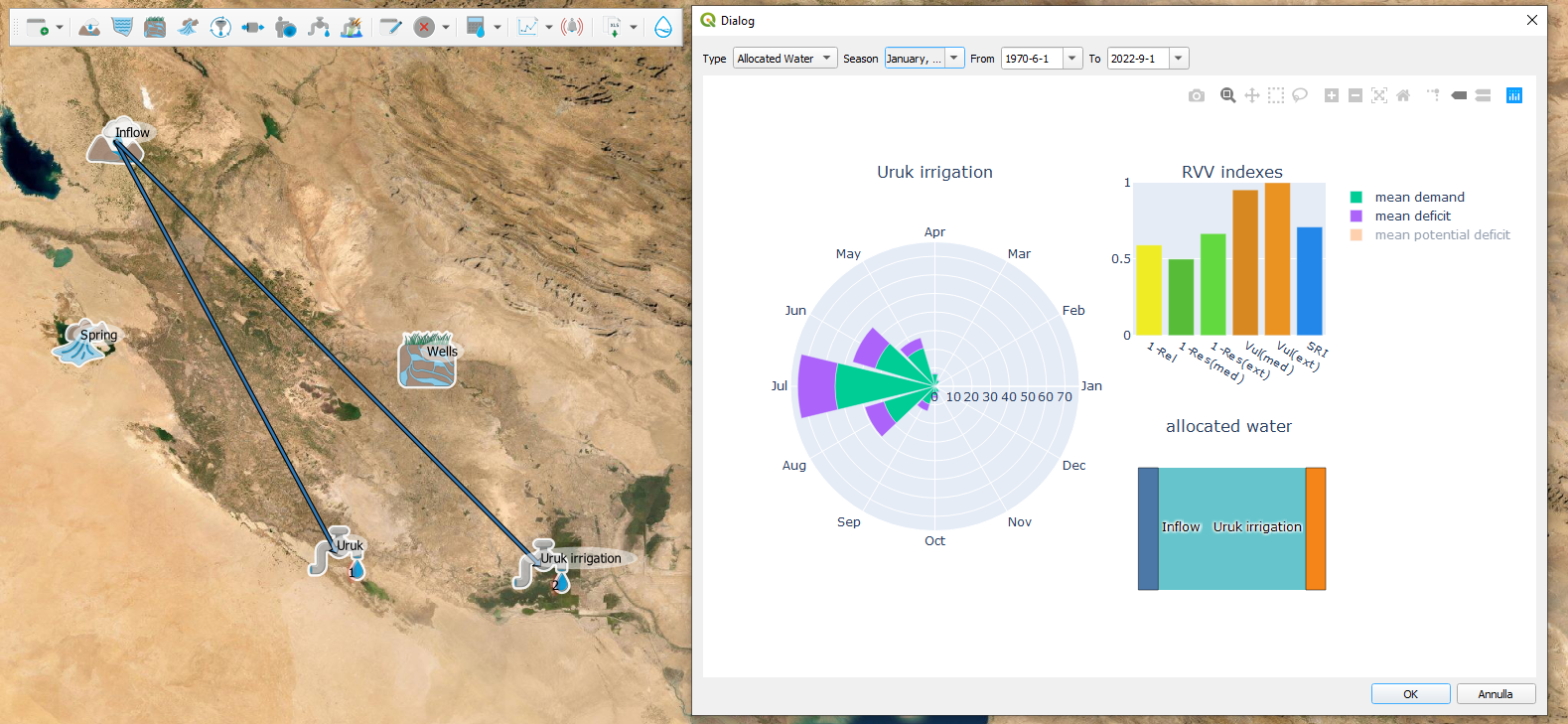
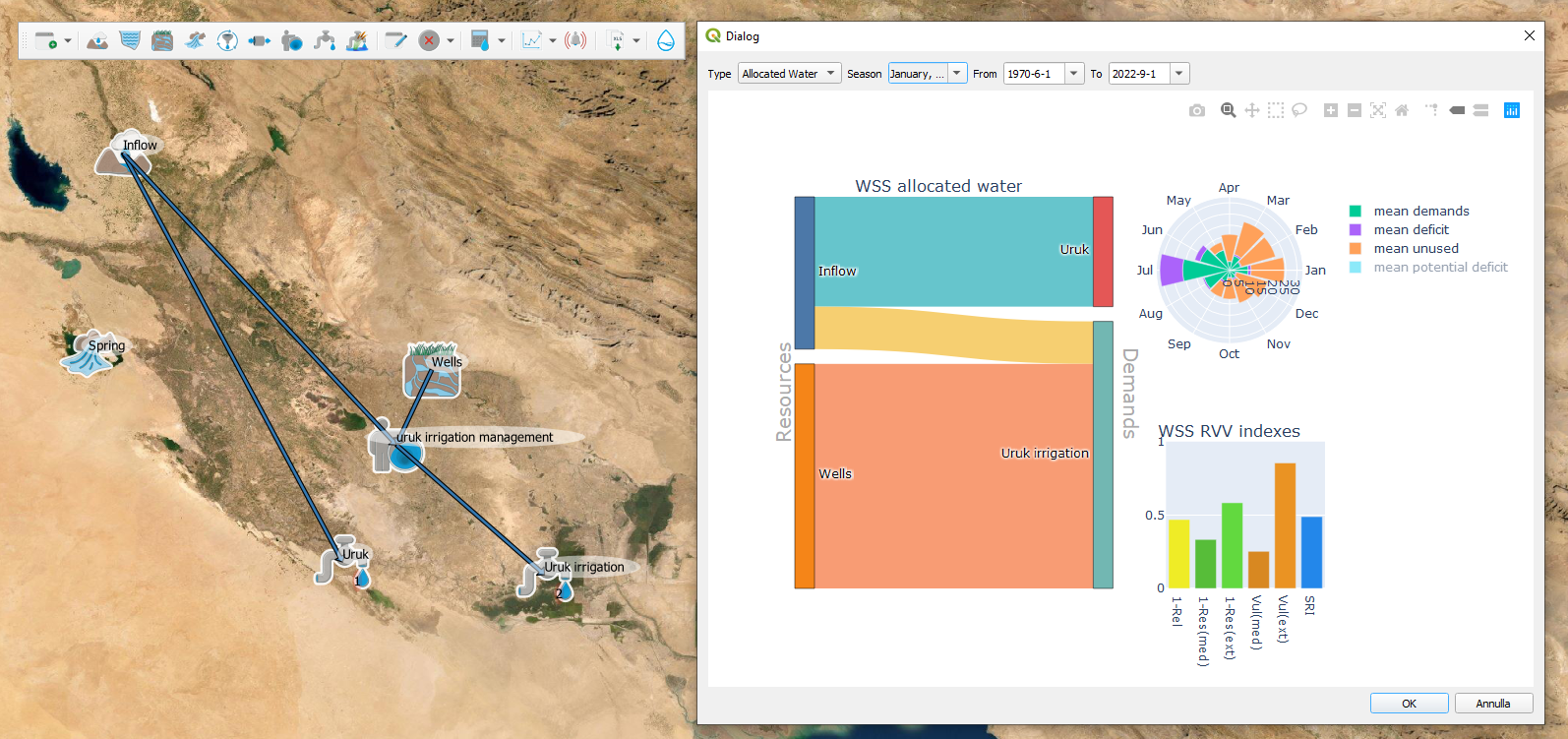
The hincast RUN has to be re-calculated to integrate the Water Supply System (WSS) modification. Once recalculated, we can select the “WSS diagnostic” among the plot, .

This gives a first overview of the implemented mono resource - multi user WSS.

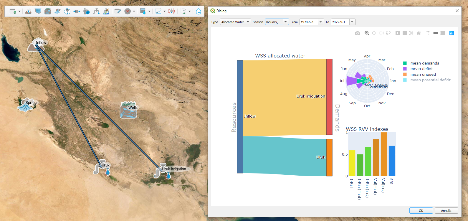
The default selection reports water allocation on the Sankey diagram (left panel). By selecting on the upper menu “deficit”, the figure will update reporting deficit flux instead of allocated water, highlighting the USER priority allocation impacts on the irrigation demand. The user can also appreciate from the drought indexes (lower right panel) how the Uruk WSS is vulnerable.

This is due to the low water availability from the INFLOW during the summer months. This can be easily appreciated by the “element diagnostic” plot applied to the INFLOW. The left panel reports monthly mean value of the element mass balance variables. Water availability is minimum during summer, while most of the winter discharge is currently unused.

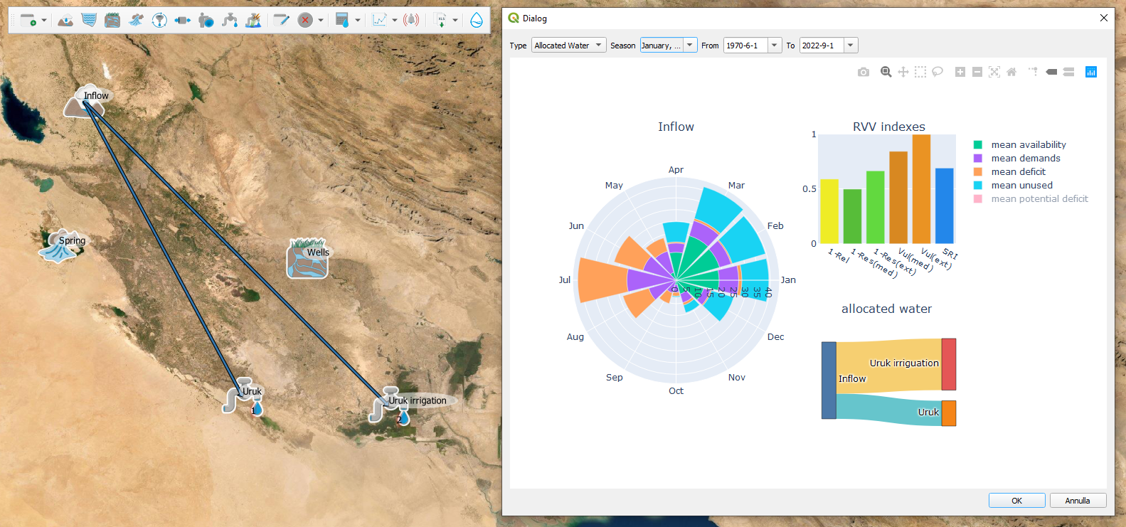
Most of the inflow summer deficit come from the hight summer irrigation demand, as it can be appreciated from the plot “element diagnostic” applied to the Uruk irrigation USER.

So the Uruk irrigation may also be addressed to the WELLS. This will result in a multi resources - mono user sub-scheme for the Uruk irrigation. To implement multi resources allocation in INOPIA, a MANAGEMENT node needs to be created, using the icone. This is necessary to set the allocation rules of the Uruk irrigation demands among the INFLOW and the WELLS. We first delete the direct connection between INFLOW and Uruk irrigation USER, using the built-in cancel tool, and clicking on the connection to be deleted .

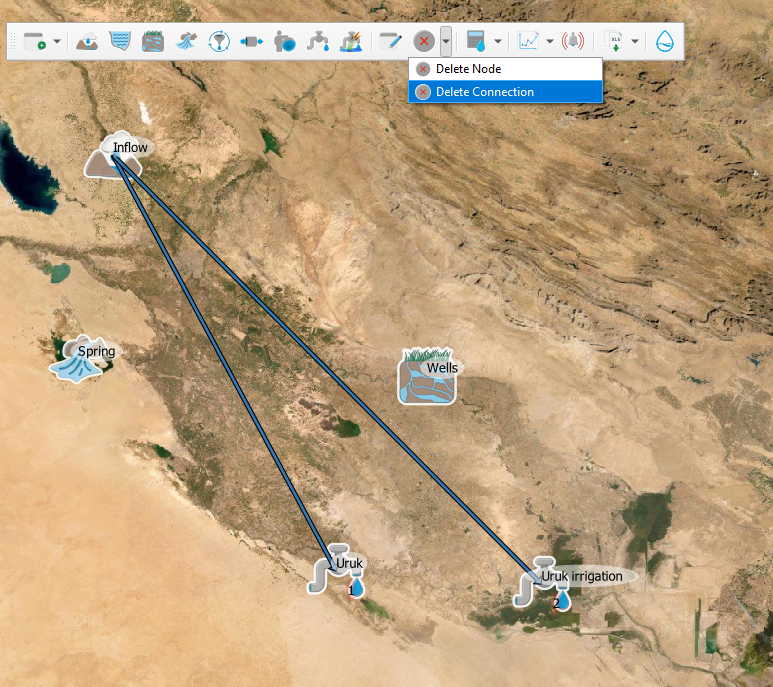
and confirm the deletion.

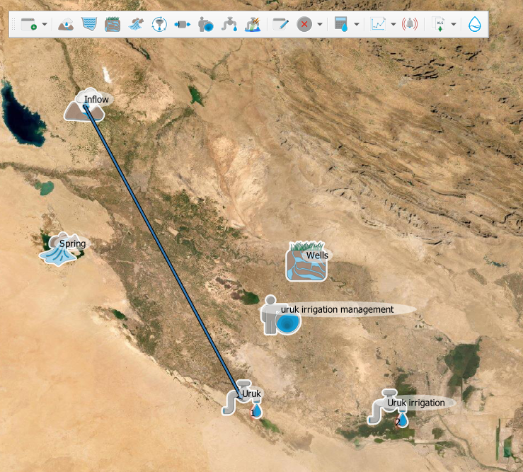
We now create a MANAGEMENT node, that we call “Uruk irrigation management”. In INOPIA, a MANAGEMENT node is always dedicated to a single USER.

and connect the MANAGEMENT node, so that both INFLOW and WELLS resources flow to the Uruk irrigation USER through the MANAGEMENT node.

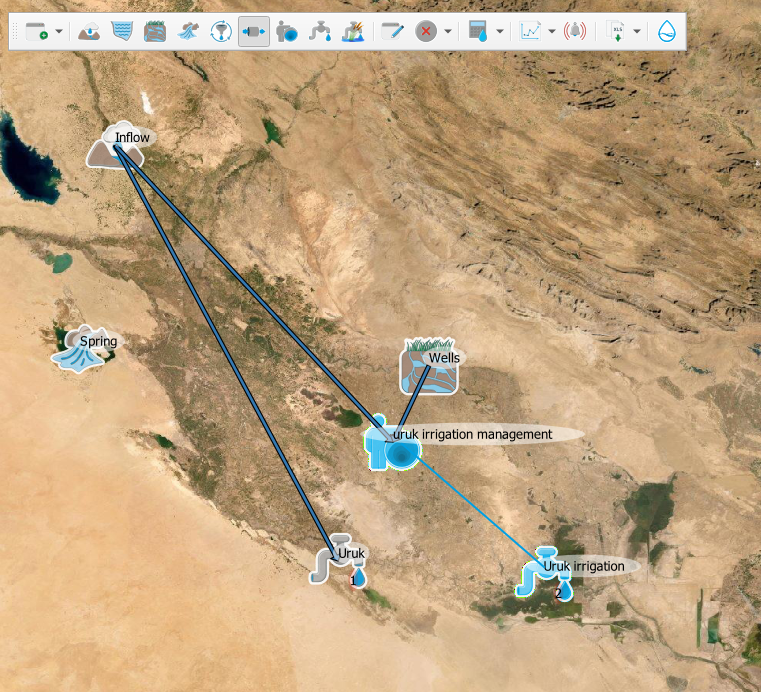
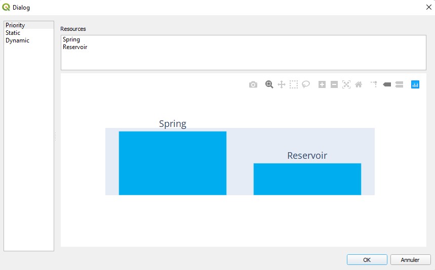
Once fully connected, the management user interface will pop-up, allowing us to select a managing rule among three built-in options: priority, static and dynamic. Those management rules are described in the INOPIA documentation. Here we select the priority rule, and make sure that the WELLS is accessed in priority, by changing the priority list with a simple click and drag (WELLS should be on the top). Clicking the OK botton will set the management rule to the current selection.

Now the Uruk irrigation will send its demand firstly to the WELLS, and secondly to the INFLOW for the Uruk irrigation multi resources - mono user sub-scheme. But as the Uruk drinking water demand is still connected to the INFLOW, the overall WSS is actually multi resources - multi user. The current allocation scheme will thus be the following:

-1. The first priority USER (Uruk drinking water) is sent to the INFLOW.

-2. The second priority USER (Uruk irrigation demand) is first sent to the WELLS through the MANAGEMENT node.

-3. If the WELLS can not fully supply the Uruk irrigation demand, the remaining demand is sent to the INFLOW.

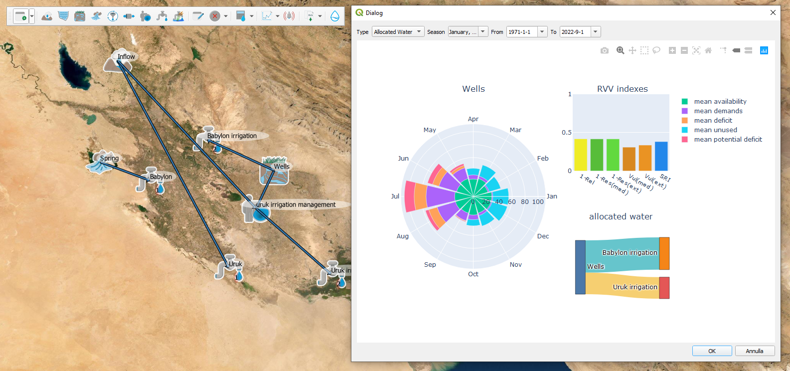
After re-calculating the hindcast run, the WSS diagnostic shows a less vulnerable WSS, as the WELLS supply most of the Uruk irrigation demand.

Chapter #3 Babylon

But Uruk is not the only USER in the region, as Babylon also has drinking water and irrigation needs. We add a priority 1 babylon USER, called “babylon”, indicating the input file “Babylon.xlsx” from the tutorial dataset, and a priority 2 babylon irrigation USER, called “babylon irrigation” indicating the input file “Babylon_irrigation.xlsx”. Babylon and Uruk drinking water demand share the same priority (as well as their respective irrigation demands).

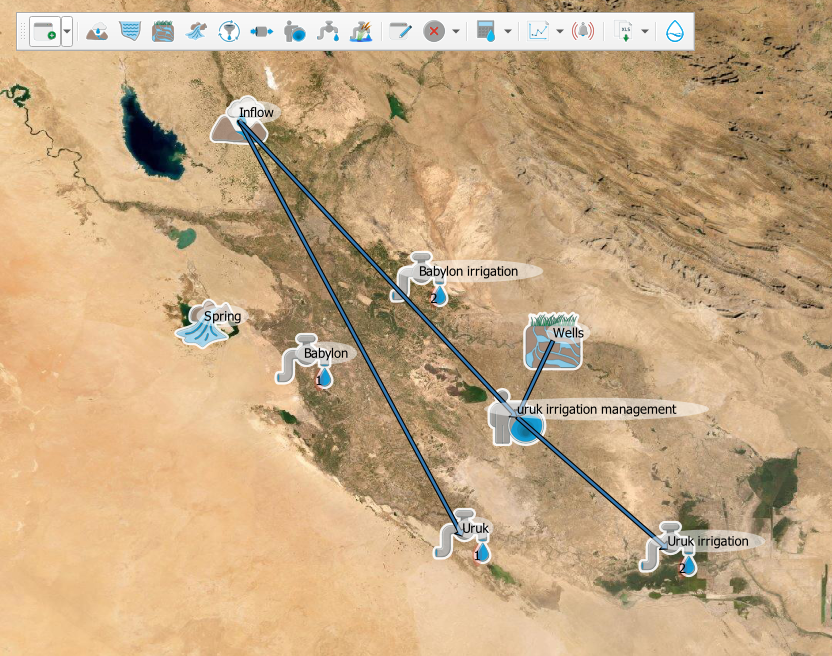
The Babylon drinking water is connected to the SPRING, while the irrigation demand is connected to the WELLS (being thus in conflic with the Uruk irrigation demand).

note that the Babylon drinking water scheme is disconnected from the rest of the WSS implemented. This is not an issue for INOPIA, as it can run more disconnected WSS within the same project

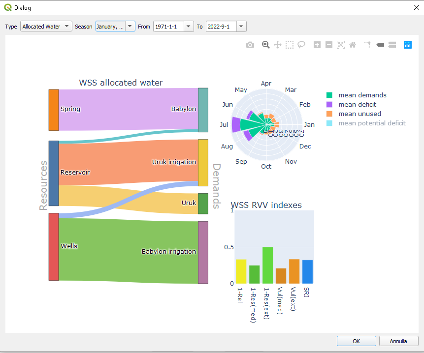
The hindcast run can be re-calculated considering the Babylon demands. It will take longer computational time, as more USERs share the same priority. A first look of the resulting mass balance can be obtained using the “WSS diagnostic” plot.

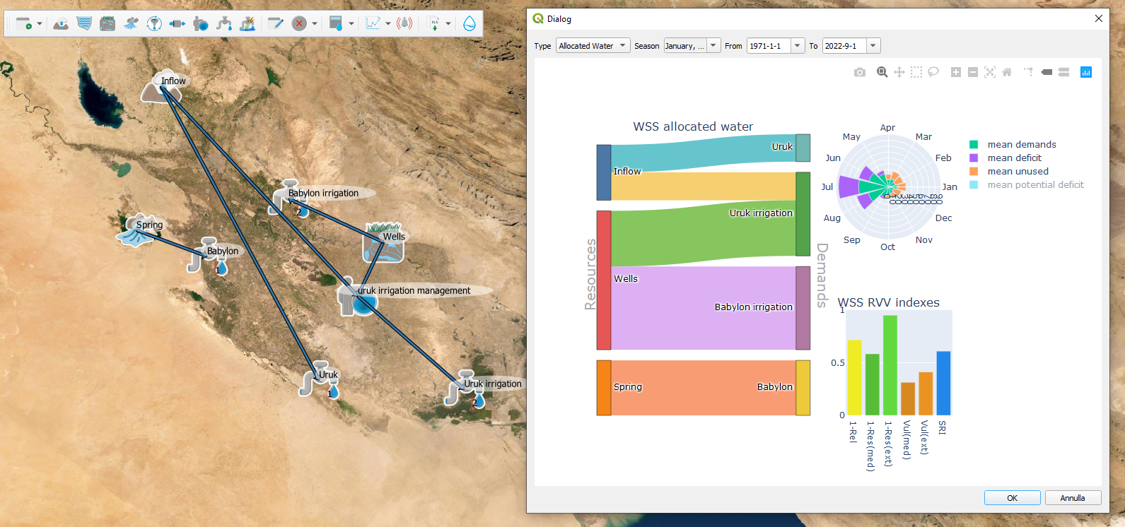
Now the WELLS resource is shared among Babylon irrigation demand and Uruk irrigation demand, which also access the INFLOW, shared with Uruk drinking water demand, while Babylon drinking water demand relies on the only SPRING resource. This result in a hight vulnerability of Babylon drinking water demand to the SPRING variability, as highlited by the “element time series” plot applied to the SPRING.

while the WELLS is now overexploited, and Uruk irrigation is still missing water during summer demand.

Chapter #4 the Dam

So they decide to build a multi purpose reservoir on the INFLOW in a common effort to supply missing drinking water to Babylon and support Uruk summer irrigation peak.

We now add the RESERVOIR, clicking on the icon and then to the location on the map. We call the RESERVOIR “Reservoir” and indicate the tutorial input file ‘Reservoir.xlsx’. The Reservoir.xlsx is filled with a maximum capacity of 150 Mm ³ and a dead volume of 15 Mm ³.

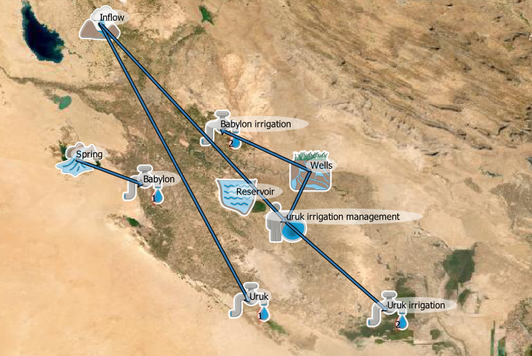
More scenarios can be considered on how take advantage of the new infrastructure. Here we will connect Babylon drinking water and Uruk irrigation demand to the Reservoir. Uruk drinking water will naturally be connected to the reservoir, as it intercepts the INFLOW. Using the we remove the current connection between the INFLOW and Uruk USER, and the connection between the INFLOW and the Uruk irrigation MANAGEMENT node. Using the we connect the INFLOW to the RESERVOIR, and the RESERVOIR to Uruk USER and Uruk irrigation MANAGEMENT node.

As the resources connected to the Uruk irrigation MANAGEMENT node has changed, the Uruk irrigation MANAGEMENT node user interface pops-up. In a collaborative framework, Uruk irrigation needs to take advantage from the RESERVOIR to release the pressure on the WELLS shared with the Babylon irrigation USER (who does not access the RESERVOIR), and shifts its management priority rule to the RESERVOIR.

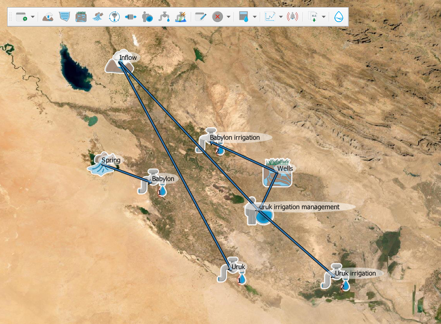
The Babylon drinking water USER is also connected to the RESERVOIR. This implies a new MANAGEMENT node, for the new mult-resources mono-user Babylon sub system. So we create a new node called “Babylon drinking water management”, cancel the direct connection from the SPRING to Babylon USER, and connect the RESERVOIR and the SPRING to the Babylon drinking water MANAGEMENT node, and finally the Babylon drinking water MANAGEMENT node to the Babylon USER. This will pop-up the new MANAGEMENT node user interface. Both to access a fresher water and to release pressure on the common multi purpose reservoir, Babylon drinking water accesses in priority to the SPRING.

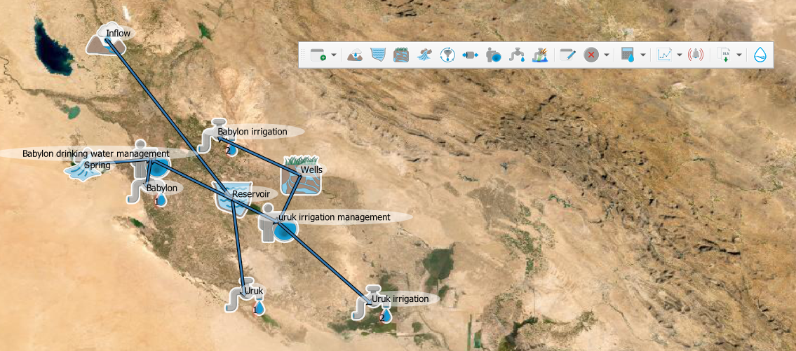
note that the Babylon drinking sub water scheme is now connected to the whole as a single complex multi-resources multi-users

Chapter #5 Coming next

In a wider collaborative framework, an ecological flow is considered to supply water to the ecosystem that previously relied on the natural INFLOW not intercepted by the RESERVOIR.

-Be prepared: To better anticipate the impact of meteorological drought on the WSS, explore RESERVOIR early warning and how the stochastic generation can improve its reliability.

-Be prepared: To better anticipate reaction of the WSS to seasonal forecast, update the hindcast to the last known monthly precipitation and test the forecast run on seasonal tendency.

-Adapt: To better anticipate the impact of climate change on the WSS, explore the supplied CIMP6 downscaled scenario run using the “Precipitation inflow_scenario.xlsx” and “Precipitation spring_scenario.xlsx” files, and test INOPIA as adaptation DSS for infrastructure scenario.

-Adapt: Test other management option or infrastructure parameter (e.g. edit “Reservoir.xlsx”) for “what if” management and infrastructural scenario on hindcast or scenarios runs. Test an alternative water resource for Uruk drinking purpose (“AtmosphericWaterHarvesting.xlsx”).